Figure 1. Holistic soil management can be used to help improve soil structure and soil quality. We explored the physical and chemical controls in Part 1 and explore the biological controls in Part 2 of this article series (all figures and tables courtesy K. Wyant.)
Management practices that improve soil health and soil quality have gained considerable attention over the past few years. If you are wondering how to get started and what to focus on, you have come to the right place! In Part 2 of this article series, I focus on how the living, biologic components of the soil, the microbes, directly impact your soil, including the structure (e.g., aggregation and pore space). My focus on bacteria and fungi in the soil is a perfect complement to Part 1 of this article series, where we explored the physical and chemical components behind soil structure. Part 1 can be found in the January/February 2021 edition of Progressive Crop Consultant.
Let us kick things off with a quick reminder of some terminology and drive home the connection between soil quality (structure) and soil health (biology).
Soil quality: This term has broad application on your farm. Soil quality refers to how well a soil functions physically, chemically and biologically and does its “job” (Figure 1). Many factors influence the soil quality on a farm and are summed up in Figure 2. In this article, we will focus on the biological management practices that maximize soil quality, expressed here as soil structure.
Figure 2. Crop productivity is influenced by several interrelated concepts, which have an impact on the soil quality of a field.
Soil health: This term refers to the interaction between organisms and their environment in a soil ecosystem and the properties provided by such interactions. When you think of soil health, think of the biological integrity of your field (e.g., microbial population and diversity) and how the soil biology supports plant growth.
There is a direct link between soil health (the living component) and soil quality (the structural component). The linkage is fungi and bacteria in the soil and the byproducts they secrete. These byproducts help restore your soil structure (Figure 3). Furthermore, well-structured soils are characterized by excellent soil health, which indicates a feedback loop between the soil biology and soil particles. But how exactly do the microbes put your soil back together?
Figure 3. The soil on the left has poor soil structure while the soil on the right has excellent aggregation and structure. The samples also have vastly different living components in the soil, as shown in the agar plates. The soil with the best aggregation is characterized by having a healthy soil microbiome (right).
Glue and Nets
Abundant and diverse soil microbial communities produce lots of “free”services for your farm soil. When your soil is healthy, microbes speed up nutrient release rates back to the crop, influence the water holding capacity of the soil, and help restore soil structure. How exactly do they go about sticking the soil together? The answer can be summed up in two terms: glues and nets.
When you have a healthy and abundant soil bacteria population, they produce a sticky, glue-like gel called extracellular polymeric substances (EPS) that forms a protective slime layer around bacteria as they grow. EPS, since it is sticky, acts as a glue for soil particles, sticking them together and improving overall soil structure.
Another important group of soil microbes, called fungi, is most known by its aboveground structures like mushrooms. However, most soil fungi exist where you cannot see them below ground. In the soil, fungi produce millions of miles of microscopic threads called hyphae. These structures help fungi find resources and grow. The threads also help to capture and tie soil particles together like a net, which improves soil structure. Now that you know the connection between your soil biology and soil structure, let us turn our attention to management practices that can help optimize the contribution of microbes to improving your farm soil (Table 1).
Soil Biology Management Guidelines
Feed the Soil Biology
This might seem like an obvious management choice, but this practice is often missed in the yearly crop plan. Your soil is teeming with fungi and bacteria and they are ready to go to work for you. The problem? They are starving and will go dormant on you until conditions improve. Research shows that farm soils are generally low in the food stuffs that microbes like to eat, and that food scarcity will limit the activity of your soil biology. The answer? Provide them with a regular installment of something they like to eat to keep their populations up. You have many choices, including microalgae, molasses, fish emulsions, etc.
Add Soil Biology
Another option is to add biology to the soil. I do not have space to cover all the products out there, but the main concept is to provide selected species of bacteria or fungi to the soil and put them to work for you. Keep in mind that the inoculant must stay alive to get the benefit you are looking for. This can be quite a challenge considering how sensitive microbes are to changes in temperature and humidity from shipping to storage in the farm shop to field application. If you choose this option, make sure your product is viable and high quality when going out into the field.
Mulches and Compost
This practice is like the first management suggestion but provides more of a “slow release” food source for the microbes. Not all the carbon in plant mulch and compost is available as microbial food. Instead, it must be chemically and physically broken down before the microbes can take advantage of it. Another advantage is that mulches and compost provide a nutrient source to the soil. A potential disadvantage here is that mulches and compost can contain excess salts and weed seeds if not prepared correctly.
Reduce Tillage and Improve Soil Biology
Field activities like tillage can be hard on your soil biology, particularly the soil fungi. For example, when a disk moves through the field, it not only slices through the soil (what you want to happen) but it also slices and dices through all the fungi threads you are trying to grow (what you do not want to happen.) This unintentional result can have a severe impact on the biological contribution to soil structure. Moreover, excessive tillage can crush and compact your soil structure, which can set you back from a physical management perspective. Reducing tillage, therefore, can improve your soil structure on two fronts. Talk about a 2-for-1 deal!
Cover Crops and Soil Biology
The cover crop, usually grown in between the rows of permanent crops (e.g., trees and vines) or in the ‘off-season’ for annual crops, can be used to help feed soil microbes. Cover crop roots secrete carbon substances, called exudates, which can help boost the soil fungi and bacteria when a crop is not in the ground. Keeping your soil alive year-round is key to optimizing the biological contribution to soil quality. Fine root hairs can also tie soil particles together, improving soil structure and quality. Another two-for-one deal!
Testing for Soil Biology
No doubt you are familiar with soil tests from your favorite agricultural laboratory. Traditional soil tests have mainly focused on measuring the chemical constituents of the soil (e.g., nitrate, phosphate, etc.) or the physical aspects of the soil (e.g., soil texture, cation exchange capacity). However, as useful as these tests are, they fail to explain how “alive” the soils are. There is good news though! Many laboratories are starting to offer soil health testing services which can help you get a better understanding of the biological components of your soil. Certified Crop Advisors (CCA) help guide growers through which test to order and, more importantly, help them interpret it. Common tests include measurements of carbon dioxide respiration, extraction of DNA for microbial community analysis and even direct counting of fungi and bacteria populations. There are many choices and sound advice from an experienced crop advisor that can help direct you down the right path and reduce the learning curve.
Conclusion
Biological factors can have a profound impact on overall soil structure and, thus, the soil quality of the field. Generally, poorly structured soils have a difficult time supporting optimized crop growth due to the severe reduction in water storage capacity, low oxygen, surface crusting and seed bed issues, accumulation of salinity, etc. If the soil looks like the example on the left side of Figure 3, it may be well worth your time and money to start implementing soil biology improvement practices as outlined in this article and revisit some of the physical and chemical practices discussed in Part 1 of this series. I strongly recommend that you put your field detective hat on to diagnose why your field is not performing as expected. A bit of detective work beforehand can pay off in turning your field around and using your input dollars most effectively.
Dr. Karl Wyant currently serves as the Vice President of Ag Science at Heliae® Agriculture where he oversees the internal and external PhycoTerra® trials, assists with building regenerative agriculture implementation and oversees agronomy training.
A combination of early weed control combined with in-season weed control was the most successful at controlling weeds and enhancing alfalfa yields.
Good stand establishment is critical for productivity of an alfalfa field both in year one and in subsequent years. Weed competition during stand establishment may be irreversible because it can reduce alfalfa root growth and lead to thinner alfalfa stands and lower forage quality. Thus, it is important to have good weed control during alfalfa stand establishment.
This project evaluated the efficacy of weed control options for both conventional and organic growers. Pre-plant mechanical cultivation and glyphosate spray were evaluated with the goal of providing regionally relevant information about an integrated weed management tool for improved stand establishment.
Methods
Six treatments (Table 1) were replicated three times in the field. Main plots were a pre-plant treatment (either no pre-plant treatment, pre-plant tillage or pre-plant glyphosate). Additionally, half of the plots received later in-season treatment (Table 1): either no treatment or Raptor application in-season after the crop had emerged.
This field was planted in the spring in the Sacramento Valley of California. Weeds were germinated with winter rains. On some plots (treatments 3 and 6), pre-plant glyphosate was sprayed on plots on January 31, 2020 at a rate of three pints glyphosate/acre. On other plots (treatments 2 and 5), mechanical cultivation was implemented on February 11, 2020 once the soil was dry enough. This cultivation was very shallow (top few inches of the soil) to avoid bringing new weed seeds to the soil surface.
Alfalfa seed was flown on the field on March 4, 2020, and the field was then ring-rolled to cover seed and get good seed-to-soil contact. The field was then irrigated for germination a week later. In-season weeds were controlled on some of the plots (treatments 4, 5 and 6) with a tank mix of Raptor (Imazamox Ammonium Salt) at 6 fl oz per acre and Buctril (Bromoxnil) on April 25, 2020.
Data Collected
Baseline weed counts were taken on January 29, 2020 from all plots before treatment implementation but after weed germination. Individual broadleaf weeds and grasses + sedges were counted in three random 20×20 cm quadrats per plot. Plants were counted on this date because weeds and alfalfa plants were small and percent cover would not have captured potential differences.
Weed counts were taken an additional three times between planting and first cutting from all plots. In-season weed counts were taken as percent cover in which the area of the quadrat was broken up in percent covered with broadleaves, grasses + sedges, bare soil and alfalfa. On April 9 and May 14, 2020, weed counts were taken in three random 20×20 cm quadrats per plot, and on June 8, 2020, percent cover was observed in three random square-meter quadrats per plot. The larger quadrat was used for percent cover on June 8 because alfalfa and weeds were tall at this time and the meter by meter square allowed for more accurate representation of each plot.
Plots were hand harvested on June 8, 2020 prior to first cutting by the grower, which occurred on June 10. Two square-meter areas of each plot, which were representative of the larger plot, were cut. Yield biomass was separated into weeds and alfalfa, dried, weighed separately and then converted to a pounds dry matter/acre basis.
Finally, on June 23, 2020, following first cutting, alfalfa stand counts were taken in all plots by counting the number of alfalfa plants in three 20×20 cm quadrats.
Baseline and Early Weed Counts
The first weed counts (January 29, 2020) collected before treatment implementation showed the average count for grasses + sedges for all plots was zero at this count. For broadleaves, there were no significant differences by treatment, but there were significantly more weeds in the side of the field with no in-season control compared to the side where Raptor was applied in-season.
April 9, 2020 Weed Counts
Grasses + sedges: There were not many grasses or sedges in the field.
Broadleaves: There were significantly less broadleaves in the plots that had pre-plant weed control (glyphosate or tillage).
Alfalfa: Alfalfa plants were small at this counting date; however, there were significant treatment differences with the pre-plant weed control treatments having more alfalfa than the control.
May 14, 2020 Weed Counts*
Grasses + sedges: There were not many grasses or sedges in the field.
Broadleaves: There were significantly less broadleaves in the plots that had pre-plant weed control (glyphosate or tillage) and in the plots that had Raptor applied in-season.
Alfalfa: There was significantly more alfalfa in the plots that had pre-plant weed control (glyphosate or tillage) and in the plots that had an in-season herbicide.
*Data not shown
This photo taken at harvest shows how heavy the weed pressure was even in plots with glyphosate or tillage pre-plant that did not have in-season herbicide application.
Broadleaf Weeds Dominated at First Cutting
There were significantly more broadleaf weeds in the plots that had no pre-plant weed control (glyphosate or tillage) (Figure 1). Additionally, the plots that had Raptor applied in-season reduced broadleaf weeds down to negligible levels compared with no in-season treatment (Figure 1). There were not many grasses or sedges in the field; however, there were more grasses in the side of the field with no in-season herbicide application.
Alfalfa Stand
There was significantly more alfalfa at first cutting in the plots that had pre-plant weed control (glyphosate or tillage) and in the plots that had an in-season herbicide (Figure 2). Weeds in the no pre-plant treatment essentially killed many of the young seedlings due to weed competition. This is a key issue since early growth and establishment of alfalfa seedlings sets the stage for vigorous growth over many years of production. This is demonstrated by the number of alfalfa plants in a 20×20 cm quadrant after first cutting (Figure 4). There were significant differences in the alfalfa stand after first cutting. With regard to pre-plant treatments, both glyphosate spray and tillage pre-plant significantly increased alfalfa stand compared to the plots with no pre-plant treatment.
Enhanced Yields
Alfalfa yields were near zero for the plots where early control was not applied (Figure 4). Additionally, yields were improved over 90% when an in-season weed control was applied (Figure 4). This yield data is only for the first cutting of the stand, not for the full first year of production. There were significant differences in alfalfa yield between pre-plant treatments and plots that had no pre-plant weed control (Figure 3). Both the glyphosate and tillage pre-plant treatments increased yields. In addition, the Raptor spray significantly increased yields compared to plots without in-season control.
A combination of early weed control combined with in-season weed control was the most successful at controlling weeds and enhancing alfalfa yields.
Biomass was separated into alfalfa (Figure 3) and weeds after plots were hand-harvested. Alfalfa and weeds were then weighed separately by plot. There were significantly more weeds by weight in the side of the field that did not get the herbicide spray in season compared to the side that did get an herbicide spray. However, within one side of the field (Raptor or not), there were no significant differences by pre-plant treatment. In other words, even though there was more alfalfa in the plots with pre-plant weed control, there were also more weeds. The photo taken at harvest show how heavy the weed pressure was even in plots with Glyphosate and tillage pre-plant that did not have in-season herbicide application.
When comparing plots with the same pre-plant treatments with or without in-season herbicide spray, plots that were tilled pre-plant did not have significantly different stand counts regardless of in-season herbicide treatment. However, within the plots that were sprayed with glyphosate pre-plant, those that also were sprayed with Raptor in-season had significantly higher alfalfa stand counts than those without in-season control.
Conclusions
The data shows that controlling weeds prior to planting, either with shallow tillage or an herbicide spray (glyphosate), will reduce weed pressure, increase yields and lead to a stronger alfalfa stand after first cutting. There were also differences between plots that got an in-season herbicide and those that did not. Yields were highest in plots that had both pre-plant weed control and an in-season herbicide. The plots with the highest stand counts after first cutting were also the plots that had both pre-plant and in-season weed control. However, the stand in the pre-plant treatment plots that did not have an in-season herbicide application still had relatively high alfalfa stand counts after first cutting. This means that with early effective weed control, the alfalfa stand may be more robust for future cuttings, even if weed pressure was high initially. As shown in the provided photos, the alfalfa was robust in the understory of the canopy, even when broadleaf weeds were very large. By first cutting, many broad leaf weeds had gone to flower, so they likely would not return after first cutting. However, when included in the harvest, these weeds reduce quality and price of the hay and also contribute seed to the weed-seed population in the field.
Ideally, both pre-plant and in-season weed control would be implemented to get highest yields, quality, a vigorous stand and ensure animal safety. However, growers (particularly organic) may be able to do a pre-plant tillage to control weeds and establish a good alfalfa stand, accept some yield reduction and additional weed pressure leading up to first cutting and then have a strong alfalfa stand for subsequent cuttings.
The author would like to thank the California Alfalfa & Forage Association for funding this project and River Garden Farms for their collaboration on this project
Stand count data was collected after first cutting (see results in Figure 4.)
Plant tissues pruned from the trees are typically flail mowed for reincorporation into the orchard floor. Nitrogen incorporated in this biomass will be released by mineralization (courtesy E. Fichtner.)
Nitrogen management plans (NMP) for California olive orchards are essential for the Irrigated Lands Regulatory Program and can increase net return. A good NMP has the potential to increase yield, improve oil quality and mitigate biotic and abiotic stresses while reducing nitrogen losses from the orchard.
Olives differ from other orchard crops in California in that they are both evergreen and alternate bearing. Individual leaves may persist on the tree for two to three years. Leaf abscission is somewhat seasonal, with most leaf drop occurring in late spring.
Rapid shoot expansion occurs on non-bearing branches during the hottest part of the summer (July/August) on ‘Manzanillo’ olives in California. The fruit on bearing branches limits current-season vegetative growth. Olives bear fruit on the prior year’s growth, and the alternate bearing cycle is characterized by extensive vegetative growth in one year followed by reproductive growth the following year (Figure 1). With bloom occurring in late April to mid-May, fruit set can be estimated in early July, allowing for consideration of crop load while interpreting foliar nutritional analysis in late July-early August.
Figure 1. Illustrative model of the alternate bearing cycle of olive (courtesy Carol Lovatt, UC Riverside.)
Critical Nitrogen Values
Foliar nitrogen content in July/August should range from approximately 1.3% to 1.7% to maintain adequate plant health. The symptoms of nitrogen deficiency manifest when foliar nitrogen content drops to 1.1% N. As leaves become increasingly nitrogen deficient, foliar chlorosis progresses from yellow-green to yellow. Leaf abscission is common at nitrogen levels below 0.9%. Nitrogen deficiency in olive is associated with a reduced number of flowers per inflorescence, low fruit set and reduced yield.
Excess nitrogen (>1.7%) adversely affects oil quality. Oil with low polyphenol concentration is associated with orchards exhibiting excess nitrogen fertility. Since polyphenols are the main antioxidant in olive oil, reduced polyphenol levels are associated with reduced oxidative stability.
Nitrogen content may impact orchard susceptibility to biotic and abiotic stresses. For example, while excess nitrogen content has been associated with increased tolerance to frost prior to dormancy, it is associated with sensitivity to low temperatures in spring (post-dormancy). High nitrogen content has also been associated with increased susceptibility to peacock spot, a foliar fungal disease on olive.
Foliar Sampling for Nitrogen Analysis
By convention, foliar nutrient analysis is conducted in late July to early August in California. Fully-expanded leaves are collected from the middle to basal region of the current year’s growth at a height of about five to eight feet from the ground. To capture a general estimate of the nitrogen status of the orchard, samples should be taken from 15 to 30 trees, with approximately five to eight leaf samples collected per tree. Leaves for analysis should only be collected from non-bearing branches. Growers may find it beneficial to make note of the ‘ON’ and ‘OFF’ status in the historical records of each block. The orchard bearing status, combined with anticipated yield and foliar analysis, will guide decisions for nitrogen applications the following year.
Nitrogen Distribution in the Tree
Over 75% of the aboveground nitrogen in the olive tree is incorporated in the vegetative biomass (Figure 2). The twigs, secondary branches, main branches and trunk account for approximately 33% of aboveground nitrogen. 23% of the aboveground nitrogen is harbored in the fruit, with the majority in the pulp (19%). Fruit is only an important nitrogen sink during the initial phase of growth. As fruit size increases, the N concentration decreases due to dilution.
Figure 2. Approximate distribution of nitrogen in the aboveground portion of olive trees (source: Rodrigues et al. 2012.)
Estimation of Nitrogen Removed from the Orchard
The easiest component of orchard nitrogen loss to estimate is the N in the harvested fruit. A ton of harvested olives removes approximately 6-8 lbs N from the orchard. The quantity of nitrogen in the fruit varies slightly between olive varieties (Table 1). Growers can use the Fruit Removal Nutrient Calculator for Olive on the CSU Chico website to gain estimates of N removal by the three oil varieties (Arbequina, Arbosana and Koroneiki) and the Manzanillo table olive. This tool was developed by Dr. Richard Rosecrance, a professor at CSU Chico, and Bill Krueger UCCE farm advisor. To access the Fruit Removal Nutrient Calculator for Olive, visit rrosecrance.yourweb.csuchico.edu/Model/OliveCalculator/OliveCalculator.html.
Pruning may generate a second component of nitrogen loss from orchards. The best practice to mitigate nitrogen loss from pruning is to reincorporate the pruned material into the orchard floor by flail mowing. The nitrogen in this organic material will gradually become available to the trees through mineralization.
In mature orchards, the wood removed by annually pruning is approximately equal to the annual vegetative growth. Consequently, the input and removal of nitrogen in vegetative growth is cyclic and almost equal in mature orchards. In young orchards, nitrogen inputs are utilized to support vegetative growth and little N is removed from the orchard in prunings or crop. During this time, nitrogen must be supplied to meet the demand to support vegetative growth. It is estimated that approximately 2.5 lbs N is required to produce 1000 lbs fresh weight of tree growth.
Nitrogen Use Efficiency
Not all the nitrogen supplied to the orchard from fertilizer and other inputs (i.e., organic matter, irrigation water) is utilized for tree growth and crop production. A fraction of nitrogen is lost from the orchard ecosystem through processes such as runoff, leaching and denitrification. Efficiency varies among orchards, with some orchard systems exhibiting higher nitrogen utilization rates than others. The efficiency generally varies from 60% to 90%. Higher values denote more efficient use of nitrogen inputs. To estimate the amount of nitrogen to supply an orchard, the demand is divided by the estimated efficiency. For example, if nitrogen demand is 50 lbs. per acre and efficiency is estimated at 0.8, then 62.5 lbs N per acre should be applied.
Nitrogen management plans are site-specific and designed to meet orchard and crop demand while reducing environmental losses. Nitrogen utilization is never 100% efficient. Nitrogen use efficiency can be maximized by minimizing losses from irrigation and fertilization practices while utilizing foliar analysis and knowledge of alternate bearing status to fine-tune applications.
References
Fernández-Escobar, et al. 2011. Scientia Horticulturae 127:452–454. Hartman, H.T. 1958. Cal Ag. Pgs 6-10. Rodrigues, M.A. et al. 2012. Scientia Horticulturae 142:205-211.
Commercial farms throughout the U.S. consistently turn out impressive yields, supplying the nation and the world with quality fruits, vegetables and staple grains. However, every year we lose organic matter and watch topsoil erode with wind and runoff. Heavy tillage, powerful biocides and mineral fertilizers support high production even on suboptimal ground. Safer crop protection products and efficient fertigation practices significantly contribute to extending the longevity of America’s agricultural lands, yet growers still struggle to maintain yields on tired, disease ridden and salt affected soils. Tillage, poor water quality, drought and soil borne disease slowly degrade soil health. Growers must invest in more water, fertilizer and pesticides to maintain their yields and crop quality on declining ground.
Organic Matter and Regenerative Practices
Healthy soils are well aerated, have good water and nutrient holding capacity, have little to no disease pressure and house beneficial microbial ecosystems. Each positive attribute relies on soil organic matter. Annual net carbon loss drives soil degradation and threatens our country’s food security. Tillage is one of the main practices contributing to organic matter loss. Turning the soil introduces an influx of oxygen, temporarily accelerating microbial activity. Bacteria and fungi, no longer limited by O2 availability, rapidly feed on organic matter, releasing carbon dioxide to the atmosphere as they respire. Tillage increases soil carbon loss beyond annual carbon gain. Reducing tillage, or converting to a no-till system, can reverse carbon loss and begin rebuilding soil organic matter. Other practices, such as cover cropping, intercropping and composting, also contribute to carbon sequestration. Specialized agronomists can assist growers in transitioning to a suite of practices to begin rebuilding soil.
No-till cover cropped systems represent the gold standard for carbon sequestration and soil health, yet logistical and economic factors prevent many growers from adopting regenerative practices. When cover cropping and no till are unfeasible, growers can support healthy microbial communities by applying carbon rich liquid amendments and biostimulants. Many organic fertilizers and amendments contain high levels of carbon, amino acids and metabolites to support beneficial microbial activity during crop growth. Carbon-rich fertilizers made from food scraps feed the soil microbiome while providing a societal benefit by diverting waste from landfills. Liquid organic fertilizers, compost and other amendments can improve soil fertility, mitigate salinity and enhance the crop’s stress tolerance. No matter where your farm lies on the sustainability spectrum, you can monitor and manage the land to improve its long-term production capacity.
Soil Health Metrics
Soil health testing can guide management decisions and gauge progress after implementing new practices. Many commercial and university labs provide soil quality panels to assess a wide array of metrics influencing the soil’s production capacity and environmental impact. Some labs offer soil health assessment frameworks that rate soil health based on results for several key indicators. Lab test results for each indicator are mathematically transformed into unitless scores reflecting the level of functionality. Scores for each indicator are combined to give an overall soil health rating. Widely respected soil health frameworks include the Cornell Soil Health Assessment, the Soil Management Assessment Framework (Andrews et al., 2004) and the Haney Test provided by Ward Laboratories.
Metrics included in the assessments vary between labs, but they all aim to include physical, chemical and biological components. Familiar measurements including pH, electrical conductivity (EC) and essential nutrients appear on soil health panels as do traditional field evaluations like water infiltration and wet aggregate stability.
Biological indicators include combustible soil organic matter, water soluble organic carbon and soil respiration. Several biological indicators must be viewed together to accurately interpret field conditions. For instance, increased microbial respiration does not always indicate improved soil health. High respiration rates combined with high organic matter likely indicate good soil health, but when the soil shows high respiration and low organic matter, the microbes may be burning soil carbon faster than it can be captured. Respiration that outpaces carbon sequestration leads to organic matter loss and soil degradation.
Advances in Biological Testing
Other biological metrics provide insight into nutrient cycling, disease pressure and crop stress tolerance. Enzyme analysis indicates the microbial community’s capacity to mineralize N, P, K and micronutrients. Pathologists can diagnose fungal, bacterial, nematode and viral pathogens so that growers can choose the right fumigants and crop rotations to keep disease pressure in check.
Phospholipid Fatty Acid Analysis (PLFA) helps determine the abundance and types of microbes in the soil. Identifying some of the beneficial microbes helps us predict the soil’s ability to inhibit disease, enhance crop growth and increase nutrient availability. Recent advances in genomics offer exciting opportunities to sequence all the DNA found in a soil sample and map microbial community composition and functioning. Genomics offer a more comprehensive analysis of microbial community than PLFA can provide. Tracking shifts in the microbiome may help determine how land management influences the soil’s trajectory towards improved sustainability.
Choosing Soil Health Indicators
Healthy soils share many common characteristics, but growers may prioritize some attributes over others depending on their needs. Growers can select soil health indicators relevant to their unique goals, production system, climate and soil type. Farmers converting to no-till can monitor progress by measuring organic matter. Those who continue tilling but begin cover cropping may not observe significant OM increases, but they might find decreased compaction and improved soil aggregate stability. Biostimulant and organic amendment efficacy may be measured by analyzing enzymatic activity and changes in the soil microbiome.
Soil health tests are accessible, affordable and offer practical insights into how farming practices affect the soil’s long term production capability. Track progress by annually measuring soil health indicators most likely to change according to the management practices implemented. Every farm can contribute to agricultural sustainability by adopting simple practices like applying carbon-based amendments or launching advanced regenerative programs such as no-till and intercropping. Soil health can also improve by knocking out disease pressure with soil fumigation and allowing beneficials to repopulate. Soil health tests can guide management decisions at every level to ensure that your effort and investment brings in quality crops every year.
Eryn Wingate is an agronomist with Tri-Tech Ag Products, Inc. in Ventura County, California. Eryn provides soil health and nutrient management consulting services to support quality crop production while meeting sustainability and environmental protection goals.
Citations & Resources
Andrews, S.S., Karlen, D.L., and Cambardella, C.A. 2004. The soil management assessment framework: a quantitative soil quality evaluation method. Soil Science Society of America Journal 68: 1945-1962.
Moebius-Clune, B.N. et al. 2016. Comprehensive Assessment of Soil Health – The Cornell Framework Manual, Edition 3.1, Cornell University, Geneva, NY.
Figure 2. Symptoms of grapevine trunk diseases on mature vines: a) classic dead arm symptoms of Botryosphaeria dieback disease; b) wedge-shaped canker characteristic of Botryosphaeria dieback; c) Eutypa dieback include stunted shoots with necrotic leaves; and d) canker and internal necrotic wedge-shaped staining in cross section of cordon characteristic of Eutypa dieback.
Grapevine trunk diseases (GTDs) are currently considered one of the most important challenges for viticulture worldwide. These widespread damaging diseases are caused by a broad range of permanent, wood-colonizing fungal pathogens, which primarily gain entry into grapevines via pruning wounds. GTDs can also reside latently within tissue as part of the normal grapevine microbiota, and environmental factors may trigger their switch to pathogenic.
The economic impact of GTDs can be significant in both young and mature vines, with Black foot disease and Petri disease being predominant in young vines. In mature vines, Esca (Figure 1), Botryosphaeria dieback (Figure 2a and 2b), Eutypa dieback (Fig. 2c and 2d) and Phomopsis dieback are damaging and referred to as canker diseases due to characteristic cankers they cause in vines. Other major symptoms of their presence include poor vigor, leaf chlorosis (Fig. 1a), berry specks and shoot and tendril dieback. Perennial cankers cause spur, cordon and trunk dieback and ultimately result in death of the entire vine.
Figure 1. Symptoms of esca vine decline: a) classic leaf stripe symptoms of esca; b) cross-section showing central white rot and canker on esca infected vine; and c) black spot and sectorial necrosis of esca-infected vine.
The majority of the fungal pathogens responsible for GTDs produce overwintering fruiting structures containing the infectious spores of the pathogen. These overwintering structures can be found on the bark surface of infected vines as well as on pruning and harvesting debris on vineyard floors. Another source of GTD fungal inoculum (spores) is from other woody perennial crops such as nut trees which are known to be infected by GTDs.
Under conducive environmental conditions, largely precipitation events, the fruiting bodies release fungal spores which land on exposed pruning wounds, causing infection and thus completing their life cycle. Research has identified that the majority of spore release in California occurs during winter following precipitation (December to February), which also overlaps with pruning timing, thus creating a window for GTDs to infect vines. With this knowledge, pruning wound protection strategies alongside cultural practices are the best strategies to mitigate GTDs. Cultural practices are focused around sanitation, including using clean material when establishing a new vineyard, removal of pruned and infected material and pruning dead shoots, spurs and cordons below symptomatic tissue. Delayed pruning after the high disease pressure period has passed is another good option in California to mitigate GTD infection.
The most effective way to protect pruning wounds from airborne fungal spores of GTDs is to apply registered chemical and/or biological pruning wound protectants. Ideally, these protectants should be applied shortly after pruning and in a dry weather window to avoid rain washing the solution away. The damaging effects of GTDs on vineyard longevity are likely to be reduced significantly if protectants are adopted when vines are young and subsequently applied annually.
Commercial chemical protectants such as a combination of Rally and Topsin M have been shown to be effective in controlling GTDs. With a need for sustainable alternatives, there is huge interest in the research, development and use of biological pruning wound protectants. Biological pruning wound protectants exploit beneficial micro-organisms that possess either natural antagonistic activity or compete with the pathogen by colonizing the pruning wound faster to provide protection from GTD pathogens. Several commercially available beneficial microorganisms, including Trichoderma spp. and Bacillus spp., have been shown to provide protection against GTDs (Brown et al. 2020; Kotze et al. 2011; Halleen et al. 2010; John et al. 2008). As well as being an alternative to fungicides, it is thought that biologicals could provide prolonged protection once they have colonized the pruning wound.
Table 1. List of all treatments used in the study, including their active ingredient, manufacturer and application rate.
Methodology
This comprehensive study was performed to evaluate a variety of registered and experimental chemical and biological agents to protect pruning wounds (Table 1) from the fungal pathogens Neofusicoccum parvum and Eutypa lata, which are aggressive causal agents of the GTDs Botryosphaeria dieback and Eutypa dieback, respectively. This study was set up in both a wine grape and table grape commercial vineyard in Sacramento County (cv Cabernet Sauvignon) and Kern County (cv Allison), respectively.
All study vines were pruned (one foot long) in February (Figure 3a), and within 24 hours of pruning, the liquid protectants were sprayed with a one-liter hand-held spray bottle on the pruning wound until runoff (Figure 3b). All protectants were prepared according to their label recommendations. The following day, canes treated with a chemical protectant were inoculated with roughly 2000 spores of either N. parvum or E. lata. Canes treated with a biological protectant were inoculated with the same amount of spores of either N. parvum or E. lata seven days after treatment application (Figure 3c). The positive control treatment had sterile distilled water applied to wounds and was inoculated with the same amount of spores of each pathogen. Eight months after inoculation, treated canes were collected and brought to the lab for further evaluation. Each cane was split with a knife longitudinally (Figure 3d) and segments were excised and plated on a growth medium to confirm the pathogen that was inoculated (Figure 3e). After incubation for 5 to 14 days at room temperature, recovery of fungal pathogens was recorded by their morphological characteristics. The efficacy of the treatments controlling the GTDs was calculated as the Mean Percent of Infection (MPI) using the following formula: Number of GTD-infected samples (canes from which the pathogen could be re-isolated)/total number of canes inoculated x 100.
Figure 3. a) Spur pruning of vines in February 2020: b) application of protectants; c) inoculation of pruned canes with GTDs; d) treated canes split longitudinally; and e) isolated segments cultured on growth media.
Results
Our results from both field studies show that Biotam, a Trichoderma-based biological product, was the superior protectant overall, providing a consistently high level of pruning wound protection compared to the water-treated, inoculated positive control. In the Sacramento County trial, Biotam application resulted in an MPI of 5% and 0% for E. lata and N. parvum, respectively, compared to the water-treated, inoculated positive control with an MPI of 40% and 70% for E. lata and N. parvum, respectively (Figure. 4a and 4b). In Kern County, Biotam application resulted in an MPI of 0% and 10% for E. lata and N. parvum, respectively, compared to the water-treated, inoculated positive control with an MPI of 25% and 45% for E. lata and N. parvum, respectively (Figure 5a and 5b). This shows that Biotam is capable of providing simultaneous pruning wound protection against multiple fungal pathogens of GTDs, which is often challenging for protectants to achieve.
Another Trichoderma-based biological product, Vintec, was also effective at protecting wounds. Application of Vintec (2.8 oz/A) resulted in an MPI of 15% and 5% for E. lata and N. parvum, respectively, in Sacramento County (Figure 4a and 4b, see page 50) and an MPI of 5% and 10% for E. lata and N. parvum, respectively, in Kern County (Figure 5a and 5b).
Figure 4. Evaluation of treatments for pruning wound protection of E. lata (a) and N. parvum (b) in Sacramento County.Figure 5. Evaluation of treatments for pruning wound protection of E. lata (a) and N. parvum (b) in Kern County.
Our results also showed that the chemical protectants Topsin M + Rally and Luna Sensation were effective at providing simultaneous pruning wound protection of E. lata and N. parvum in both Sacramento and Kern County trials. Application of Topsin M + Rally resulted in an MPI of 10% for both E. lata and N. parvum in Sacramento County (Fig. 4a and 4b, see page 50) and an MPI of 5% and 10% for E. lata and N. parvum, respectively, in Kern County (Figure 5a and 5b, see page 50). Several naturally occurring biocontrol agents, including Trichoderma hamatum (UCD 8717), Aureobasidium pullulans (UCD 8189) and Bacillus sp. (UCD 8745), that were identified in California vineyards were also performing very well compared with other commercially available products (Figure 4 and 5).
In conclusion, our 2020 field trials have shown that several biological and chemical treatments can provide efficient protection of pruning wounds of grapevine against one or more fungal pathogens responsible for the major grapevine trunk diseases (Esca, Botryosphaeria dieback and Eutypa dieback). Moreover, improving accurate diagnosis of GTDs will be essential in determining an effective product.
References
Brown, A.A., Travadon, R., Lawrence D.P., Torres, G., Zhuang., and Baumgartner, K. 2021. Pruning-wound protectants for trunk-disease management in California table grapes. Crop Protection, 141.
Halleen, F., Fourie, P.H., and Lombard, P.J. 2010. Protection of grapevine pruning wounds against Eutypa lata by biological and chemical methods. A. Afr. J. Enol. Vitic. 31: 125–132.
Kotze, C., Van Niekerk, J., Mostert, L., Halleen, F., and Fourie, P. 2011. Evaluation of biocontrol agents for grapevine pruning wound protection against trunk pathogen infection. Phytopathol. Mediterr. 50: 247–263.
John, S., Wicks, T.J., Hunt, J.S., and Scott, E.S. 2008. Colonisation of grapevine wood by Trichoderma harzianum and Eutypa lata. Aust. J. Grape Wine Res. 14:18-24.
Irrigation is probably the most powerful tool a winegrape grower has in their tool box. Intelligent use of irrigation can control canopy size, manage vine stress, manipulate berry size, improve wine quality and conserve water. The key to achieving a grower’s viticultural goals through irrigation is data-driven scheduling to determine when and how much to irrigate.
The tools growers have available for irrigation scheduling generally fall into five categories: soil-based, plant-based, weather-based, remote sensing and visual assessment of the vine’s water status.
Soil-Based Methods and Technologies
Soil moisture sensors are an effective way of measuring how much water is in the soil, where it is in the profile and how and when the vine is taking up that water. Another benefit of soil moisture sensors is the ability to measure the effect of winter rain on the soil profile
For the best resolution, multiple sensors are needed per block reflecting soil types and topography. The key is placing sensors in locations which are representative of larger areas. Soil maps can help identify the best locations. Ideally, a soil map was made prior to vineyard installation. Mapping can still be done after installation with the help of a professional agricultural soils expert. Identifying representative areas within a vineyard can also be done using Normalized Difference Vegetative Index (NDVI) mapping. These maps identify areas of weak or excessive vigor. Those areas should be avoided as locations for sensors.
The best depths for sensor placement can be determined by taking soil cores with a hand auger. Look for changes between soil horizons which might impact water holding capacity. Depths should represent rooting depths and just below to monitor deep percolation. Place the sensor in the vine row approximately 18 inches from the vine trunk and four to six inches from the emitter.
Types of soil moisture sensors include quantitative technologies such as time domain transmissometry, capacitance measurements, time domain reflectometry and qualitative methods such as matric potential. Each has its advantages and disadvantages in terms of cost, soil volume measured and ease of installation. No one type of sensor is ideal for all situations, so some research and ground truthing against other methods like visual assessment is required to find the best fit for your particular vineyard.
Plant-Based Methods and Technologies
Probably the most common method for evaluating vine water status is leaf or stem water potential using a device such as a pressure bomb. This method measures the tension (or “potential”) between the pull of water through the plant from evapotranspiration and how tightly water is held to the soil. A leaf is cut from the vine. The blade is placed under pressure forcing water back through the xylem of the petiole. The more pressure required to force the water out, the drier the vine is.
A porometer is another tool which directly measures an indicator of vine water status. Porometers provide a reading of how relatively open or closed the stomata are on the leaf. Stomata are open when there is water available for evapotranspiration. When stomata start to close, the vine is protecting itself from drying out—a sign of stress. A sensor is clipped to a leaf blade and a measurement is taken automatically.
An indirect measurement of stomatal closure can be done with an Infrared thermometer. Transpiration cools the surface of the leaf, making it cooler than the ambient air temperature. As stomata close, the temperature of the leaf blade increases. Readings are taken by simply pointing an infrared thermometer at the canopy. This method is simple, quick and generates good quality data that is easy to interpret when analyzed over time.
Weather-Based Methods and Technologies
While not a direct measure of vine water status, weather-based methods allow for data-informed scheduling decisions for the vineyard as a whole. By estimating how much water vines have transpired, a grower can decide how much water to put back into the soil, or not, in the case of deficit irrigation. This is done by estimating the daily water loss of the vine using evapotranspiration (ET) rates. The baseline for comparison is the reference ET, also called ETO or “full ET”. The California Irrigation Management Information System (CIMIS) maintains remote stations throughout California to provide reliable estimates of ET. Many weather stations available today also estimate ETO.
Grapevines do not transpire at the full ET rate, so a crop coefficient (KC) is required to better reflect how the vine is behaving under these conditions. Essentially, the more canopy, the more water is transpired by the vine. As canopy size varies during the course of the growing season, the ratio of water transpired by the vine to reference ET changes. Therefore, the crop coefficient needs to be calculated at multiple times during the season. Calculating the crop ET (ETC) uses the equation ETO × KC = ETC.
KC is determined by measuring the percent of the vineyard floor shaded at solar noon. This can be done with a gridded board to estimate the width of the shade and the percent of gaps in the shaded area. The percentage of shaded floor area is then used in the following equation to calculate the crop coefficient: KC = Percent shaded area × 0.017
Using ETC is especially helpful for successful deficit irrigation. A crop coefficient for deficit irrigations, called KRDI, can be calculated by multiplying KC by the percent deficit desired using the equation KC × %RDI target = KRDI. This gives the grower confidence that they are hitting their specific target for deficit irrigation taking current weather conditions into account.
An example:
The percent of vineyard floor shaded is 25%.
This gives a KC of 0.425.
If the RDI target is 75% the KRDI is 0.319.
If the ETO rate for the week is two inches, 0.638 acre-inches should be applied to maintain vines at their current water status.
Remote Sensing
Remote sensing using the Normalized Difference Vegetative Index (NDVI) is a powerful tool as it provides a literal picture of vine vigor across a large area to a high degree of resolution. Maps are created by flying over the vineyard with a drone or fixed wing aircraft. Cameras on the aircraft record the amounts of near infrared and red wave lengths reflected by the vineyard canopy. NDVI is calculated using an equation that compares these wavelengths. The resulting numbers correlate to the relative photosynthetic activity of the canopy which is directly tied to vine water status.
Visual Assessment
Purely qualitative practices for assessing vine water status are commonly used by growers. One can simply look at the appearance of vines searching for tell-tale signs of stress without the need for any devices. This is an excellent way of ground truthing other methods.
Vine response to stress can readily be seen in the growth pattern of shoots and angle of leaf blades. When tendrils extend far beyond the shoot tip, the vine is growing rapidly and is under no stress. As the soil and vine begin to dry out, tendrils become shorter.
Shoot tips are another good indicator. The state of a shoot tip can be determined by folding the last fully opened leaf up toward the tip. If the shoot tip extends past the leaves, it is active. If the folded leaves cover the shoot tip, it has stopped growing. Eventually, the tip will die altogether.
Leaves provide another clue to vine stress. Under stress, leaves begin to droop. Leaves on an unstressed vine will form an obtuse angle to the petiole. As stress progresses, this angle becomes less and less until it is acute.
Using visual inspection of the vine successfully requires many years of experience to perfect. Combining experience with quantifying technology may give the grower more confidence that their “read” of the vines is correct. One serious drawback of relying solely on looking at vines for indicators of stress is that there is a delay between the onset of stress and the symptoms becoming apparent in the state of the canopy. Overshooting a stress goal under RDI can be difficult to recover from, especially during late season.
Consider using a combination of at least two different types of irrigation scheduling methods as each measures different variables and provides a different viewpoint of what is happening in the field. The vine’s response to irrigation depends on soil physics, changes in weather patterns year to year, vine age, crop load, canopy size and disease status. Taking all those variables into account is challenging even with the best tools. The more tools in the tool box, the better equipped the grower is to harness the power of well scheduled irrigation.
Figure 1. Grape powdery mildew occupies a niche bathed in sunlight, and it senses and uses light to direct its development. Researchers are learning new ways to use that evolved process against the pathogen to suppress disease (all photos courtesy D. Gadoury.)
Global winegrape production is largely based upon the production of the European winegrape Vitis vinifera, a host species comprised of cultivars that are all highly susceptible to infection by the grape powdery mildew pathogen Erisyphe necator as well as several other fungal and oomycete pathogens. Irrespective of the center of origin of Vitis vinifera or the major pathogen groups, the global ubiquity of both the host and various pathogens is now a fact faced by grape and wine producers everywhere.
In particular, fungicidal suppression of grapevine powdery mildew is problematic. Resistance to many FRAC classes, including sterol demethylation inhibitors (DMI), strobilurins, benzimidazoles and succinate dehydrogenase inhibitor (SDHI) fungicides is sufficiently widespread that the forgoing classes are no longer effective in some viticultural regions. Organic production systems are also threatened. There are very few practical organic options for controlling powdery mildews. Many organic options entail undesirable non-target effects or are marginally effective. Additionally, many viticultural regions are located in Mediterranean climates with little rainfall during the crop production season. All of the foregoing creates the present situation: grapevine powdery mildew predominates as the principal threat to healthy fruit and foliage worldwide.
UV Light to Suppress Pathogens
Nearly all of the biomass of powdery mildews is wholly external to the host (Figure 1). They live in a world bathed in sunlight throughout the disease process. With the exception of the walls of their overwintering structures (chasmothecia), they possess none of the pigmentation that would offer protection from biocidal wavelengths of the solar spectrum (wavelengths of UVB between 280 and 290 nm.) Powdery mildews are favored by shade and repressed to some degree by direct sunlight exposure. They persist in the above niche due in part to their ability to repair UV-inflicted damage to their DNA through a robust photolyase mechanism driven by blue light and UVA.
In 1990, we began work that led to the use of germicidal UVC lamps to suppress E. necator. The treatments were effective, but UVC also damaged the vines, and the technology was never widely adopted (Figure 2). It took 20 years before a critical breakthrough by a Ph.D. student in Norway (Aruppillai Suthparan) fundamentally changed how we could use UV light against plant pathogens. He found that if UV light was applied during night hours, we could use much lower doses than were required during daylight. That breakthrough largely resolved the issue of plant damage at the high UV doses required for daytime applications. Today, UV technology for plant disease suppression is being investigated by several working groups. Most exploit the link between darkness and the inability to withstand exposure to UV. When damage to pathogen DNA during darkness is not repaired within four hours, it is usually lethal.
Figure 2. Researchers at Cornell used UVC applications to suppress grape powdery mildew as early as 1991. While effective, the treatments also caused damage to both the leaves and fruit. A breakthrough discovery several years later by a PhD student in Norway unlocked the key to effective treatments without plant injury.
The UV spectrum used in such studies has ranged from a UVB waveband between 280 to 290 nm into the UVC range produced by low pressure discharge lamps yielding a peak output near 254 nm. Reduction of the severity of several powdery mildews has been attributed to direct damage to the pathogen by UV exposure. UVC has been reported to be directly inhibitory to Botrytis cinerea on strawberry (Janisiewicz et al. 2016). In contrast, pathogens other than powdery mildews have been suppressed by exposure of their hosts to UV prior to inoculation, possibly due to enhancement of host resistance.
The adaptation of nighttime UV treatments to commercial field plantings has necessitated the development of UV arrays powerful enough to apply effective doses at speeds that allow the equipment to complete treatments during the available night interval, often in late spring and early summer during some of the shortest nights of the year. Remember: we need about four hours of darkness after UV exposure in order to achieve the maximum suppression. A tractor-drawn UVC apparatus described in a report by Onofre et al (2019) was developed to suppress strawberry powdery mildew. This apparatus contained two hemicylindrical arrays of UVC lamps and was the basis of a later array design fitted to an autonomous robotic carriage produced by Saga Robotics, LLC. UVC treatments applied once or twice weekly at doses ranging from 70 to 200 J/m2 effectively suppressed strawberry powdery mildew (Podosphaera aphanis) to a degree that equaled or exceeded that of some of the best available fungicides.
The potential for nighttime UV treatments to eliminate the threat posed by E. necator could greatly reduce the need for fungicide applications. In regions with higher rainfall and multiple fungal pathogens, the potential for nighttime UV treatments to remove the threat of powdery mildew would improve options for the remaining members of the pathogen and pest complex, such as downy mildew (Plasmopara viticola), bunch rot (Botrytis cinerea) and various arthropod pests.
For all of the foregoing reasons, our objectives in the present study were to 1) Determine the potential of nighttime UV applications to suppress grapevine powdery mildew; 2) Determine if UVC at disease-suppressive doses and frequency of application has any deleterious effects on vine growth, yield or crop quality; and 3) Determine if nighttime UV applications targeting powdery mildew have effects on other selected pests or diseases of grapevine.
In summary, the mechanism underlying the success of nighttime UV applications is related to how pathogens deal with naturally-occurring ultraviolet light from the sun. Shorter-wave UVB and UVB both damage DNA in all living organisms. Exposure to UV causes thymine base pairs in the DNA to bind together, changing the genetic code to genetic gobbledygook. Pathogens sense visible light, but they also possess evolved systems that can repair the foregoing damage to their DNA caused by incoming UV. We now know that those biochemical and genetic repair systems are recharged by blue light and UV-A, and are reduced by red light and darkness. This photolyase-based repair mechanism effectively “unglues” the thymine base pairs as fast as they are created by UV, but the repair mechanism does not operate at night.
Lamps producing UV light have been commonly available for over 75 years. Those that produce an effective wavelength and are powerful enough to be practically used against powdery mildews produce either UVC (100 to 280 nm) or UVB (280 to 315 nm). Both UVC and UVB affect DNA in the same way by the aforementioned creation of thymine dimmers. UVB poses less potential to harm plants, and may therefore be preferred for static and permanent installations in greenhouses. However, with precise dosing, UVC can be used safely on even UV-sensitive crops.
Low-pressure discharge lamps are the most common available technology. Low-pressure discharge UVC lamps are generally clear quartz-glass tubes containing a small amount of mercury vapor. Passing an electric arc through this vapor results in the efficient production of a narrow waveband centered on 254 nm, which is excellent for germicidal applications. UVB low-pressure discharge lamps are similar, but incorporate a fluorophore powder coating on the inside of the tube. When this is struck by the internally produced UVC, the fluorophore absorbs the UVC and emits the longer wavelength UVB. This process is also relatively inefficient, and nearly 95% of the usable germicidal energy is lost in the conversion from UVC to UVB. So, low-pressure discharge UVC lamps can produce much more usable power than comparably sized UVB lamps. While UV LEDs are available, they are presently far too expensive and underpowered to be useful for treating crops.
Results Adapted to Grapevine
Field trials for suppression of strawberry powdery mildew were initiated in Florida in 2017. Weekly applications of UVC provided suppression of foliar powdery mildew across the duration of the experiment that was substantially better than that provided by the best fungicide treatment in the trial, which was a combination of two materials sold under the trade names Quintec and Torino. We also confirmed in parallel measurements that the UV treatments did not reduce plant size or the yield of harvested berries. Continued trials on field plantings of strawberries duplicated the efficacy of the 2017 trials.
In our initial trials, we used a tractor-drawn array (Figure 3). Additional trials adapted modified designs of the original tractor-drawn array to an autonomous robotic device (Figure 4) manufactured by SAGA Robotics, a Norwegian company collaborating with our research group in developing this technology for multiple crops. The use of a robotic carriage provides additional flexibility in nighttime applications. At temperate latitudes, the duration of night near the summer solstice can be less than eight hours, leaving only about four hours during which the UV treatments could be applied with optimal effect. In situations where employing nighttime labor to make applications split over several relatively short night intervals would be problematic, an autonomous robotic device offers a practical alternative.
Figure 3. Tractor-drawn UVC array used in the first large-scale field trials on strawberries. Side-by-side arrays allowed two rows to be treated in each pass.Figure 4. Thorvald, an autonomous robotic device developed in collaboration with SAGA Robotics in Norway, can carry and power the same UV array used in tractor drawn devices.
In 2019, we came full circle and were ready to resume UV treatments on grapevine. As in our work on strawberry, we began by using a UV array and tractor-drawn carriage. UV Treatments were applied once per week at 100 or 200 J/m2 to Chardonnay vines that received no other fungicide treatments. Laboratory experiments had indicated that the UV doses used would stop 80% to nearly 100% of the conidia of E. necator from germinating. The incidence and severity of powdery mildew was assessed on leaves and fruit of UV treated vines, vines treated with an effective conventional fungicide and completely untreated vines. 2019 was a moderately severe year for powdery mildew.
Both the 100 J/m2 and 200 J/m2 UVC treatments significantly but equivalently reduced the severity of powdery mildew on berries compared to the untreated vines, albeit not to the degree provided by the standard fungicide treatments (Figure 5). What surprised us was that both the 100 J/m2 and 200 J/m2 UV treatments also suppressed foliar downy mildew (Plasmopara viticola), and did so better than the fungicide standard (Figure 6). Laboratory studies indicated that the suppression of the downy mildew pathogen was due to a pre-inoculation increase in host resistance. This was distinct from the impact of UV on powdery mildew, which was primarily a direct effect of UV on the pathogen itself. However, in our 2020 trials, weather conditions were especially conducive to downy mildew, and the level of suppression of downy mildew from UV was only around 50%. That’s helpful, but it is nowhere near acceptable commerical control. So, we obviously have more work to do in this area.
Figure 5. Efficacy of UVC treatments for suppression of powdery mildew on Chardonnay grapes, 2019.Figure 6. Foliar severity of grapevine downy mildew on Chardonnay vines treated weekly with UVC at 100 or 200 J/m2 compared to a standard fungicide treatment and untreated control.
The 2019 trials produced another surprise: the UV treatments effectively suppressed sour rot (Figure 7). This disease is a complex mess involving bacteria, fungi and fruit-feeding insects. We still don’t understand how UV is accomplishing this reduction, but given that there are very few effective means to suppress sour rot, any efficacy due to UV treatments is worth further investigation.
Figure 7. Suppression of sour rot on Vignoles grapes treated with UVC at 200 J/m2 compared to a standard fungicide treatment and untreated control.
In addition to suppressing plant pathogenic fungi, UV treatments can also suppress populations of phytophagous mites (Figure 8). A number of studies have noted that UVB and UVC treatments can kill eggs of spider mites and European Red Mites. In addition to these effects, our preliminary trials indicate that the UV treatments can also alter behavior of adult mites, reduce egg laying, and reduce fecundity of the generation of surviving mites that emerge from UV treated eggs.
Figure 8. The egg and immature stages of mites are susceptible to UV treatments, and this technology is now widely used, particularly in the Netherlands for suppression of mites in greenhouses and high tunnel production systems.
As in our strawberry work, we eventually wanted to adapt the tractor-drawn grape UV array to a robotic carriage, and our partnership with SAGA robotics made this possible (Figure 9). The navigation autonomy of the SAGA robot (Thorvald) is capable of tracking within a few centimeters of the trellis center at operational speeds between 1.25 to 2.5 mph. We evaluated UV doses between 100 J/m2 and 200 J/m2 at frequencies of either once weekly or twice weekly. All of the evaluated doses significantly suppressed powdery mildew on both fruit and foliage, and the twice-weekly 200 J/m2 treatment provided control that was superior to the fungicide standard (Figure 10).
Figure 9. A tractor-drawn UVC lamp array used to treat grapevines at Cornell Agritech, and the same array carried by the autonomous robot Thorvald, manufactured by Saga Robotics.Figure 10. Efficacy of UVC treatments for suppression of powdery mildew on Chardonnay grapes, 2020.
What’s Next?
We are collaborating with growers and scientists at multiple locations in the U.S. and Europe, including Bully Hill Vineyards in Hammondsport, N.Y.; Washington State University’s research and extension center in Prosser, and the USDA Horticultural Crops Research Center in Corvallis, Ore. as well as multiple locations in California, with designs and materials for UVC lamp arrays adapted for their vineyard pruning and training systems. These trials will be conducted over the course of the 2021 growing season. More about the autonomous robot Thorvald can be found at sagarobotics.com/. Our international working group is described on our project website: LightAndPlantHealth.org. It is a large, multidisciplinary, multi-institutional and international group representing several U.S. and overseas universities and government agencies, with industrial partnerships (Figure 11).
Figure 11. Group photo: Members of the research/extension team and advisory committee for our USDA-OREI project. Left to right: Laura Pedersen, Pedersen Farms, Geneva, NY; Eric Sideman, NOFA; Arupplillai Suthaparan, NMBU, Norway; Arne Stensvand, NIBIO Norway; Mariana Figueiro, Mount Sinai Light and Health Research Center (LHRC); Mark Rea, Mount Sinai LHRC; David Gadoury, Cornell University; Ole Myhrene, Myhrene AS, Norway; Rebecca Sideman, University of New Hampshire; and Robert Seem, Cornell University. Below (left to right), other members of the research and extension project team: Dr. Natalia Peres and PhD student Rodrigo Onofre, UFL Gulf Coast Research and Education Center; Dr. Lance Cadle-Davidson, USDA Grape Genetics Research Unit; Dr. Jan Nyrop, Department of Entomology, Cornell University and Director at Cornell AgriTech; Dr. Walt Mahaffee, USDA-ARS, Corvallis, OR; and Dr. Michelle Moyer, University of Washington, Irrigated Agriculture Research and Extension Center, Prosser.
The design of a lamp array to match a particular crop canopy and target pest biology is a critical aspect determining of the success of the treatments. Our cooperative projects with growers across the US have always involved our array designs and electronics. Some growers have designed and fabricated the various carriages for the arrays. But the UV array itself is NOT a DIY project, nor is calibration and the photobiological and epidemiological calculations that enter into calculations of a proper UV dose for specific applications. In addition to the engineering and biological considerations, both UVB and UVC can be injurious to you unless devices are properly designed and the lamps are properly shielded from direct view. No person should ever have an unshielded view of germicidal UV lamps, as there is a significant risk of eye and skin damage from exposure UVB and UVC. The protective gear that is required for safe applications is not expensive, and consists of UV-opaque clothing that covers all exposed skin, disposable gloves and a face-shield and eye protection rated for protection from UV. The arrays shown in this article also incorporate clear PVC curtains at each end of the array to limit escape of UV from the array. As would be the case with any IPM technology, UV does not pose undue risks to operators or the environment if used properly. Proper training and use protocols are the key to safe and effective applications.
Our work has been funded by competitive grants from the USDA Organic Research and Extension Initiative, and the USDA Specialty Crops Research Initiative. Additional support has been provided by the National Research Council of Norway, the New York Farm Viability Institute, the USDA Sustainable Agriculture Research and Extension Program and Bully Hill Vineyards. We work as a diverse international group to promote this research area and its applications, and to act as a resource to train others. The work spans disciplines from plant growth and photobiology to physics and lighting technology.
David M. Gadoury is a senior research associate in Cornell’s Plant Pathology and Plant-Microbe Biology Section at Cornell AgriTech, where his program focuses on pathogen ecology, pathogen biology and disease management. He leads the Light and Plant Health Group.
References
Gadoury, D.M., Pearson, R.C., Seem, R.C., Henick-Kling, T., Creasy, L.L., and Michaloski, A. 1992. Control of diseases of grapevine by short-wave ultraviolet light. Phytopathology 82:243.
Janisiewicz, W. J., Takeda, F., Glenn, D. M., Camp, M. J., & Jurick, W. M. (2016a). Dark Period Following UV-C Treatment Enhances Killing of Botrytis cinerea 3.Conidia and Controls Gray Mold of Strawberries. Phytopathology, 106(4), 386–394. https://doi.org/10.1094/PHYTO-09-15-0240-R
Michaloski, A.J. 1991. Method and apparatus for ultraviolet treatment of plants. U.S. Patent no. 5,040,329.
Onofre, R. B., Gadoury, D. M., Stensvand, A., Bierman, A., Rea, M., and Peres, N. A. 2019. Use of ultraviolet light to suppress powdery mildew in strawberry fruit production fields. Plant Dis. 105:0000-0000 (in press).
Suthaparan, A., Stensvand, A., Solhaug, K. A., Torre, S., Mortensen, L. M., Gadoury, D. M., Seem, R. C., and Gislerød, H. R. 2012. Suppression of powdery mildew (Podosphaera pannosa) in greenhouse roses by brief exposure to supplemental UV-B radiation. Plant Dis. 96:1653-1660.
Suthaparan, A., Stensvand, A., Solhaug, K. A., Torre, S., Telfer, K. H., Ruud, A. K., Mortensen, L. M., Gadoury, D. M., Seem, R. C., and Gislerød, H. R. 2014. Suppression of cucumber powdery mildew by supplemental UV-B radiation in greenhouses can be augmented or reduced by background radiation quality. Plant Dis. 98:1349-1357.
Figure 1. A front view of Oxbo over-the-row (OTR) blueberry harvester (all photos courtesy F. Takeda.)
Blueberry production acreage in the U.S. is expanding. Across the country, commercial blueberry growers are increasingly using over-the-row (OTR) mechanical harvesters (MH) to pick their blueberries for fresh market (Figure 1). Growers everywhere are experiencing difficulties in finding sufficient labor for hand harvest operations and due to the rising costs of labor. Harvesting blueberries with OTR harvesters can significantly reduce the overall cost of harvesting to a fraction of that needed for hand harvesting (HH) and workers needed for harvest operations from about 500 hours of labor per acre per year to as little as three hours of labor per acre per year. However, compared to hand harvesting, OTR harvesting causes more berry loss due to falling on the ground and green/red berries are harvested along with ripe, blue fruit.
Detailed field testing of OTR harvesters for picking blueberries for the fresh market was conducted nearly 30 years ago in Michigan. That research in South Haven, Mich. evaluated the quality of blueberries harvested by hand and by four rotary and slapper harvesters that were used by growers at that time to harvest blueberries for processing. MH blueberries were sorted at the packinghouse (Figure 2).
Figure 2. Mechanical harvesting detaches unripe green fruit and clusters that must be sorted out on the grading line.
The most significant findings were a high percentage of detached blueberries had impact damage (Figure 3) and more than 20% of detached blueberries fell on the ground. The bruise damage was attributed to iImpact to the fruit created by the rapid actions of shaking rods and detached berries landing on the hard catching surface. Those studies revealed that blueberries harvested by the machines had a high percentage of blueberries with more than 20% of sliced surface area showing bruise damage (Figure 3 and 4). Also, MH blueberries were much softer compared to hand harvested fruit. Their conclusion was that MH blueberries should not be cold-stored for more than two weeks while HH blueberries could go in controlled atmosphere storage for six weeks and air-shipped to Europe in excellent condition.
Figure 3. Bruise damage caused by mechanical harvesting makes the flesh dark and soft. Half of these berries have excessive bruising.Figure 4. Sliced examples of mechanically harvested blueberries. From left to right: Fruit with no internal bruise as indicated by no large discolored tissue; Fruit with impact damage at the stem end as indicated by discoloration inside the seed core; Fruit exhibiting damaged area from impact force to that triangular shaped, discolored section; and Discolored area has been highlighted in purple with SketchAndCalc program to calculate bruised area as 17% of the total cut surface area.
Soon after, USDA engineers developed an experimental harvester called the V45 harvester designed specifically to harvest fresh-market blueberries. It used a direct-drive shaker with an angled, double-spike-drum, a unique cane dividing and positioning system to push the canes out diagonally and cushioned catching surfaces to harvest fruit with minimum damage. With the V45 harvester design, the detached blueberries dropped less than 15 inches onto a soft neoprene sheet glued to a hard catch plate and soft sheet over the conveyor belt.
These soft surfaces reduced impact force on the fruit detached by the V45 harvester. However, gluing a soft surface onto a hard surface has proven to show little reduction in bruise damage when harvesting is performed with conventional harvesters with two vertical drum shakers and berries falling more than 30 inches. Only five V45 harvesters were sold by the now defunct B.E.I Inc. (South Haven, Mich.), although it was thought to have good fruit selectivity (low green fruit removal) compared to slapper models, little ground loss (fruiting cane pushed away from the crown) and superior quality over existing commercial harvesters at the time with two vertical drum shakers and either a metal or hard plastic catch surface.
Sometimes, the fruit harvested by the V45 harvester had quality as good as commercially HH fruit. Its limitations were: 1) It needed to be driven much slower to avoid damaging bushes; 2) It could not harvest trellised rows or those with overhead sprinklers; and 3) It could not harvest all varieties, especially those with stiff, upright canes like ‘Jersey’ and many rabbiteye cultivars. The Fulcrum harvester made by A&B Packing Equipment (Lawrence, Mich.) has features like those of the V45 harvester.
In the last ten years or so, U.S. blueberry farmers targeting the fresh market have been facing challenging economic situations (e.g., rising cost of hand picking, shrinking labor force, global competition, etc.) They and other specialty crop farmers have a greater interest in using automation and OTR machines to harvest their crop. The authors of this article have participated in different aspects of machine harvesting and sorting of blueberries to reduce the amount of internal bruise damage and in packing line sorting technology and damage detection systems to improve the quality of packed fruit. Several blueberry MH manufacturers (e.g., Oxbo International, Lynden, Wash.; A&B Packing Equipment, Lawrence, Mich.; BSK, Serbia; and FineFields, the Netherlands) have put more efforts devoted to developing MH systems that would impart low or no bruise damage so that fruits can be packed for fresh market. Following is a summary of recent developments in MH.
Bruised Berries from Mechanical Harvesting
Most OTR harvesters currently available are better suited for harvesting processed blueberries because they can cause excessive fruit damage. However, OTR machines have been used to pick blueberries for fresh market. In these instances, the fruit should be packed and transported to consumers as quickly as possible. When blueberries are HH, typically the picker gently picks ripe fruit selectively. In Chile and China, for example, ripe berries are picked individually to obtain high fresh quality.
In the Pacific Northwest and elsewhere in North America, ripe fruit is often harvested by rubbing fruit cluster or sometimes by “tickling” them between the thumb and index finger and catching the detached berries in the palm and then placing them in a small harvesting bucket. In contrast, MH involves the shaking of the entire bush with rapid action of shaking rods to move canes back and forth. The cane movement causes ripe berries that need less fruit removal force than green/red berries to be displaced from the fruit stem (pedicel) and fall onto catching surfaces. Experienced MH operators make slight adjustments on machine settings to obtain good selectivity (minimize green/red berry removal and maximize ripe fruit removal).
The blueberry bush can range from 3 to about 6 feet tall with fruit located from the tip of the canes to branches near the ground, which causes the berries located on the top part of bush to fall as much as 50 inches. When an OTR harvester picks blueberries and fruit falls from that height onto plastic catch plates and conveyor belts, one can hear berries hitting the hard catch surfaces.
Based on this simplified description of the blueberry MH process, it was apparent that the interaction between the machine and fruit should be better understood. To do this, we used a custom-made miniature electronic sphere called the BIRD (blueberry impact recording device developed at the University of Georgia) to measure the fruit impacts during MH process in 2010 and 2011. The BIRD sensor for this study weighed 14 g. The later version, BIRD II, was built to closely approximate the size and weight of a large blueberry (9/16-in diameter and weighed 6 g) (Figure 5).
Figure 5 . BIRD II (red sphere) connected with a 4-pin connector to a laptop to charge its internal battery, initiate impact measurements or download collected data to a laptop or mobile device.
Along with documenting fruit impacts with a BIRD, a closeup video camera recorded the harvesting to pinpoint critical control points where most impacts were created. The results showed that the drop to the plastic catch plates on the harvester accounted for over 30% of all impacts on the BIRD, followed by the drop from the grading belt on the harvester into an empty lug (20%). When the lug is filled with blueberries, fruit-to-fruit impacts occur, which are much lower than when the fruit fall into an empty lug.
Impacts created by the conveyor, including secondary bounce from the catch plates, and shaking rods combined for another 25% of recorded impacts. The remaining 25% of impacts that occurred before the sphere contacted the catch plate were classified as obscured impact events which could not be identified clearly from the video and were attributed to contact with the shaking rod, branches and the vertical tunnel panels. These measurements suggested that the most significant reduction in fruit impacts could be achieved by 1) Modifying the catch plates; 2) Reducing drop heights, either by restricting bush size, placing catching surfaces closer to the fruit or decreasing drop heights at other transition points; and 3) Placing softer surfaces at the transition points (e.g., at transfer points in the fruit handing equipment on the top of platform.)
The two parts of the impacts include the number of encounters between the sphere and different surfaces of the harvester and the magnitude of these impacts. In our study, the harvesting process was documented with video that recorded time-stamped impact events with the larger, heavier BIRD I sensor. Using these parameters, the OTR MH process was divided into four phases: Phase I (detachment and falling), Phase II (fruit hitting the catch plate/conveyor belt), Phase III (elevation from the conveyor/transfer belt to the top platform and conveyance through a trash blower) and Phase IV (dropping from the conveyor belt into the lug).
Results showed that for the rotary drum shaker, the BIRD sensor recorded an average of 18 impacts in Phases I to IV. During Phase I, it is assumed blueberries detached by fast-moving harvesting rods that shake left and right, impact branches as they fall and/or are flung out to the side panel. There were about five impact events in Phase I, but magnitudes of these impacts proved to be less significant than initially assumed. In Phase II, the BIRD contacted the catch plate and usually only one or two events were recorded. The magnitude of the impacts in Phase II was extremely high compared to impacts recorded in Phases I, III and IV. Our results strongly suggested that the high impact that the falling blueberries receive at the point of contact with the catch plate injures the fruit, resulting in fruit softening and larger bruise while the fruit is in storage (Figures 3 and 4).
Further analysis was performed by dropping the large, heavier BIRD I sensor onto a hard-plastic catch plate from different heights (6, 12, 24, 36 and 48 in) (Figure 6). As expected, the impact values (peak acceleration at impact (g) increased sharply linearly with increasing drop height, ranging from 280 g at 6 in to about 800 g at 48 in (data not shown). In subsequent studies, impact measurements were made using the smaller and lighter-weight BIRD II sphere by dropping onto soft surfaces created by placing cushioned padding on top of the hard plastic plates or by suspending the soft material (no hard surface underneath.)
Figure 6. The relationship between various contact surface materials and drop height. The impacts were collected with a BIRD II sphere dropped from different heights.
A wide range of impact values were obtained depending on the hardness of the catch plate (Figure 6). Impacts greater than 200 g were recorded on hard surfaces such as a stainless-steel sheet and a plastic catch plate even when the BIRD II was dropped from a height less than 30 cm (12 in). Gluing a soft surface to a hard surface reduced impact; however, this type of surface still created high impact above a one-foot drop height such that blueberries falling 30 inches onto such a surface would still be bruised. For example, the suspended foam sheet we used in our harvest-assist blueberry picking machine in 2017 generated less than 200 g even when the drop height was 42 in, but well above the 120 g at which ripe blueberries can be bruised by impact force. Only the netted fabric that acted like a hammock produced low enough impact force and kept the blueberries from getting bruised even when the fruit was dropped from a 48-in height. Thus, it was thought that replacing the hard, plastic fruit catching and collection surfaces with soft and durable catching surface materials and plate design features that prevent soft surface from contacting any hard surfaces underneath had the potential to improve the quality of MH blueberries and reduce bruise damage associated with high mechanical impact.
In terms of mechanical impact to blueberry fruit, our research has shown that bruise damage and the loss of firmness in MH fruit can be decreased by reducing space between blueberries on the bush and the catching surface to 12 inches in the case of hard plastic fruit catching surfaces or by modifying the fruit catching surfaces to create a softer fruit landing surface. Ideally, the fruit catching surface should not exceed 120 g impact even when the BIRD II is dropped from a height of 48 in (equivalent to the distance between the top of a large mature blueberry bush and catch plates on the harvester).
The design of soft surfaces can be achieved by either incorporating netted material or a soft “rubber” sheet with no hard surfaces beneath for catching the fruit (Takeda and Wolford, U.S. Patent No. 9,750,188 and the Oxbo SoftSurface kit). For example, even with a soft surface insert in a hollowed-out plexiglass catch plate, the margins of the plate contributed to more than 20% of the exposed surface area. In addition, catch plates on the harvester overlapped with adjacent plates and rested on top of another plate. The outline of the plate below another created about 10% additional hard surfaces.
When blueberries are HH, the packout is about 95% or better and fruit usually have little or no internal bruise damage (Table 1). The packout of MH blueberries is lower and typically ranges from 70% to slightly more than 80%. The remaining 20% consists of soft, overripe and immature green- and red-colored berries.
Table 1. Effect of catch surface (hard or soft) and drop height on internal bruise damage within one day of drop and after 14 days in cold storage (32 degrees F to 37 degrees F). Bruise damage is expressed as the percentage of cut surface area indicated by dark color (see Figure 4).
Commercial packing operations, for the most part, do not check for internal bruise damage in their MH blueberries. However, close inspections of MH blueberries packed into clamshells after sorting on commercial packing lines revealed berries were bruised (Figure 3, see page 4). Our studies evaluated different catch surface designs by inserting soft, flexible material to reduce internal bruise damage. We did record improvements in packout. However, neither the improvement in packout nor berry firmness approached that of HH fruit in the case of varieties Duke, Draper or southern highbush blueberry (SHB) Optimus even when they were harvested with OTR machines equipped with soft, flexible catch surfaces. The only exception to date has been the variety Last Call, where MH produced the quality approaching that of HH berries. MH of SHB Optimus produced higher-quality packout than other SHB varieties, such as Jewel, Star and Farthing, but even Optimus should not be cold-stored for more than one week. Our studies have shown that fresh market pack-out can be increased by installing a soft catch surface on the harvester, but the quality of HH blueberries has been better.
Cultivar Susceptibility
In a study conducted in Oregon, the susceptibility of 11 blueberry cultivars to impact damage was determined by dropping the fruit from 2-, 3-, and 4-foot heights onto a hard, plastic catch plate. Bruises developed more rapidly in rabbiteye cultivars (Ochlocknee, Powderblue and Overtime) than in northern highbush (NHB) and SHB cultivars. NHB cultivars Aurora, Cargo, Draper and Last Call had the least amount of bruising after two weeks in cold storage. Blue Ribbon, Legacy and Liberty had a moderate amount of bruising.
These studies showed that simulated drop tests are useful in determining the potential of varieties for long-term cold storage and, more importantly, their potential to MH for fresh market. In a study in 2020 in Oregon, Draper and Legacy were MH with two OTR Oxbo harvesters, one fitted with and the other without the SOFTSurface kit. To date, the challenge for Oxbo Corporation and other machine manufacturers has been to procure soft materials that meet food safety standards and are durable for harvesting blueberries.
The preliminary findings of this study were: 1) Machine harvesting with the SOFTSurface kit reduced fruit internal bruise damage in both Draper and Legacy fruits compared to those harvested with the unmodified OTR harvester as shown with a laboratory test (Table 1); 2) Draper and Legacy fruit harvested with the machine fitted with the SOFTSurface kit and sampled before sorting in the packing house were firmer compared to fruit harvested by the unmodified harvester; and 3) After one and two weeks in cold storage, there was no difference in firmness of berries harvested by machines fitted with and without the SOFTSurface kit.
We found that fruit firmness-based sorting by itself may not be a good predictor of berry quality when MH blueberries are cold-stored for two weeks or more, but both Draper and Legacy blueberries picked by the OTR machine fitted with the SOFTSurface kit maintained better fruit firmness (>160 g/mm) values and lower internal bruise ratings in cold storage (Table 1). The improvements in fruit quality may well have been from a 70% reduction in hard catch surface area in the SOFTSurface kit compared to the hard polycarbonate fruit catching surfaces in the regular harvesters. A laboratory test determined the effects of dropping blueberries from different heights onto either a hard (e.g., polycarbonate catch plate on conventional harvesters) or soft catch surface (e.g., prototype SOFTSurface kit) on internal bruise development (Table 1). Blueberries were sliced to visually assess bruise damage on the day of the drop test and after cold storage for two weeks.
Young (~3-ft-tall) and mature (6-ft-tall) trellised Last Call blueberry plants were either HH or picked with a modified OTR machine. Fruit samples from both methods were manually sorted and evaluated for internal bruise damage on the day of harvest and the remaining samples were placed in cold storage. Cold-stored samples were taken out after two and four weeks and evaluated for internal bruise damage (Table 2). On the day of harvest (zero days after harvest), about 80% of blueberries showed no bruise damage, and the remainder showed damage ranging from 1% to more than 50%. There was little change in internal bruise for samples from matures bushes that were either HH or MH. However, there was a dramatic decline in the percentage of fruit with no internal damage among the samples from machine harvesting of young plants.
Table 2. Percent of blueberries in each internal bruise damage (IBD) category as affected by hand harvesting and harvesting with a modified OTR machine and the age of ‘Last Call’ northern highbush blueberry immediately after harvesting and after two and four weeks in cold storage.
Our field observations of the Last Call bushes used in this study indicated that the canes of young plants were upright during the harvest and detached fruit fell straight down. In contrast, on the taller, mature bushes, the canes had grown well above the height of the trellis and they were leaning outward at the time of harvest. This placed the fruit away from the crown and less than 30 inches above the catching surface and may have contributed to reducing mechanical impacts in terms of numbers and magnitude, thus reducing the amount of internal bruise damage.
Sorting Out Bruised Berries
Blueberry growers in the Pacific Northwest and in Chile have expressed an interest in machine harvesting blueberries for the export market. The consensus among them is that the varieties for the export market must be firm and arrive at the destination in excellent condition after more than three weeks of cold storage and a transoceanic travel period. Our machine harvesting research has consistently shown that the MH blueberries generally had more internal bruise damage and shorter shelf life than the HH blueberries.
Commercial optical sorting equipment are now available for grading blueberries. In the last three years, HH and MH blueberries have been processed on commercial blueberry packing lines in Oregon and Washington equipped with an optical sorter (e.g., UNITEC, BBC and MAF). For each packing line, samples of Draper and Legacy were taken from lugs prior to unloading onto the conveyor system, and a second group of samples were collected after the fruit had gone through the optical sorting machine. Samples from both locations were assessed for bruise damage (% bruised area). The bruise data are presented in Table 3 in which the data are expressed in terms of how the samples were distributed (e.g., blueberries with no damage to those that were severely bruised.) The analysis indicated that sorting by optical sorters did not remove blueberries with moderate to severe internal bruise damage.
Table 3. Determination of internal bruise damage in machine-harvested Draper and Legacy blueberry samples collected from packing line locations either before or after inspection with an optical sorter. Samples were sliced through their equator and the bruised area was assessed visually as the percentage of sliced area and converted to a value between 0 and 5 using a 5rating scale: 0= no bruise, 1= 1% to 5% bruised, 2= 6% to 10%, 3= 11% to 20%, 4=21% to 50% and 5= greater than 50%.
Next, we compared the blueberry fruit firmness value with the area of internal bruise damage on the sliced surface. One would likely assume that softer fruit will have more bruise damage. Our results and those from a report by Chilean researchers showed that this was not the case as shown by the low correlation coefficient (r-value) for these two fruit quality parameters. Whether the fruit had been collected from the packing line before or after the optical sorting machine, the correlation coefficients for berry firmness and bruise damage were less than 0.4 in NHB cultivars. This suggested that optical sorters in commercial blueberry packing houses were not effective in removing blueberries with internal bruise damage.
Once more in the laboratory, we conducted drop tests in which HH Duke blueberries were dropped from a height of 62 inches to ensure that the samples would be bruised. A hyperspectral imaging system was used to locate and quantify bruise damage in each whole fruit (25 berries at a time). We then measured fruit firmness with a FirmTech II at the site of the bruise impact as determined by the imaging system. Then, the same fruit was rotated and additional firmness measurements were taken at 90 and 180 degrees from the bruised site.
The analysis showed that at the site of the bruise damage, the average fruit firmness was 149 g/mm. However, at the sites that were 90 and 180 degrees from the impacted location, the firmness was greater than 162 g/mm. This meant that a lower firmness value was detected when the damaged area was purposely used to determine firmness, resulting in a much higher r-value between fruit firmness and internal bruise damage values. Fruit that were firm at the time of packing (e.g., >180 g/mm value using a FirmTech II instrument) were found to have internal bruise damage exceeding 15%. In the near future, our research team will sort MH blueberries with this imaging system to separate whole unbruised and bruised blueberries and conduct postharvest quality evaluation for unbruised and bruised MH blueberries to determine the shelf life of each group with an eye toward exporting MH blueberries to distant Asian markets. Of course, taking this non-destructive imaging system from the laboratory bench to integrating it into commercial optical sorting machines for IBD detection and sorting is a challenge facing the machine manufacturers.
Conclusions
More blueberries for fresh market are being machine harvested.
Machine harvested blueberries have more internal bruise damage.
On-going research is developing a better understanding of what causes bruising and working with harvest machine manufacturer to reduce bruise damage.
New sensor technologies for blueberry sorting could assist in reducing bruised berries in fresh packs.
Our research has shown that to make MH more profitable for blueberry growers, the current OTR harvesters must be modified to reduce impact damage and ground loss. Cultivars with superior machine harvestability are being released by blueberry breeding programs, and research must continue to develop equipment capable of harvesting blueberries with less bruise damage. The sorting system on the packing line for MH fruit must be improved with a greater precision to eliminate fruit with severe internal bruise damage. This would ensure that the quality of MH blueberries going into clamshells would be as good as HH fruit. Blueberry growers in some regions can then contemplate having MH blueberries packed for export. Also, proper training and pruning of blueberry bushes to maintain a small crown can increase MH efficiency. These changes will help in making small, incremental improvements in increasing pack-outs and fresh quality of packed blueberries.
Finally, in order for MH blueberries to have quality that is as good as HH fruit, the blueberry industry needs to be willing to make changes by growing superior varieties, modifying how blueberry bushes are grown and harvested, and improving how the fruit is sorted. This will take a concerted effort from growers, breeders, horticulturists, engineers and supply chain specialists. These changes could lead to blueberry fields that look different from what we see today, with radically different ways of harvesting blueberries and technological advancements for sorting blueberries with the goal of improving the quality of MH blueberries going into clamshells.
In terms of harvesting and packing technology, it is envisioned that U.S. blueberry growers will be using robotic harvesting systems in the field or in warehouses with specialized automated or semi-automated harvesting machines that will avoid damaging berries, have better selectivity to reduce green berries picked and sort out over-ripe and diseased berries in the field. In packing houses, new non-destructive technologies are needed that will be capable of analyzing the blueberry fruit surface and below the skin and sort fruit for quality (large size, high sweetness, flavor, bloom, no bruise damage and color). These advances will facilitate market segmentation and high prices as one U.S. and several European blueberry distributors are doing already with HH blueberries.
This research was supported in part by the U.S. Department of Agriculture agencies (Agricultural Research Service (Project No. 8080-21000-028, National Institute for Food and Agriculture (Agreement No. : 2008-51180-19579 and 2014-51181-22471), Agricultural Marketing Service (FY 18 Oregon Department of Agriculture SCBG to WQY and FY18 Washington SCBG to LWD), U.S. Highbush Blueberry Council, Chilean Blueberry Committee and Naturipe Farms Blue Challenge.
Our gratitude goes to blueberry growers and packers in Waldo, Fla.; Alma and Homerville, Ga.; South Haven and Grand Junction, Mich.; Kingsburg and Stockton, Calif.; Hillsboro, Independence and Roseburg, Ore.; and Burlington, Prosser, Lynden and Sumas, Wash., and in Chile who provided much needed in-kind support to the harvest project. A special thanks goes to Oxbo International Corporation which has collaborated with the group since 2014.
Authors are employees of USDA-ARS (FT, fumi.takeda@usda.gov) Oregon State University (WQY, wei.yang@oregonstate.edu), University of Georgia (CL, cyli@uga.edu), Washington State University (LWV, lisa.devetter@wsu.edu) and University of Florida (SS, sasa@ufl.edu and JW, jgrw@ufl.edu).
Mention of trade names or commercial products in this publication is solely for the purpose of providing specific information and does not imply recommendation or endorsement by the U.S. Department of Agriculture. USDA is an equal opportunity provider and employer.
Potassium demand in wine grape vineyards is highest during fruit ripening in mid- to late summer. Applications made after bloom jumpstart enzymatic action, including photosynthesis. Deficiency symptoms usually occur early into mid-summer, starting with color loss at leaf edges (photo courtesy Wilbur-Ellis Ag.)
Nutrition is an important part of managing a wine grape vineyard since it impacts vine growth, crop yield, berry composition and, ultimately, wine quality.
Grape variety, rootstock, vine age, soil type and irrigation supply along with yield and production and quality expectations all figure into a summer nutrition program.
Dr. Raj Madam, branded technologies manager for Wilbur-Ellis Agribusiness, said applications of macronutrients, nitrogen, phosphorus, potassium and magnesium as well as application of micronutrients must be timed and delivered to match plant demands. Excess vegetative growth resulting from over-application of nitrogen can have a negative effect on sugars and berry color.
Vine function is affected when essential nutrients are not supplied. Severe nutritional deficiencies can be seen first in leaves. Unless corrected, the shoots, canes and fruit may also develop symptoms. Visual symptoms and leaf and soil analysis are all useful to evaluate nutritional status.
Dr. Madam said vines use 100 to 150 units of N per year, with 25 units per application. Applications of NPK are generally made just before bloom. This timing corresponds to a vine’s timing for N at fruit set just after bloom. Grapevines use nitrogen to build essential compounds including proteins, enzymes, amino acids, nucleic acids and pigments, including chlorophyll and anthocyanins of fruit.
Vine demand for potassium is highest during fruit ripening in mid- to late summer. Applications are often made after bloom when they serve to jumpstart enzymatic action including photosynthesis. Deficiency symptoms usually occur early into mid-summer, starting with color loss at leaf edges.
Vines use potassium to form sugars and starches for the synthesis of proteins and for cell division. Potassium also neutralizes organic acids and regulates the activity of other mineral nutrients in vines.
The form of potassium applied is also important for uptake by the vines, Dr. Madam said. The acetate form, such as the Wilbur-Ellis product Till-It® 70, is the most soluble for vine uptake, Dr. Madam said.
Magnesium is a micronutrient often overlooked in vineyard nutrient management, he added. It is the central component of the chlorophyll molecule, the green pigment responsible for photosynthesis in green plants. Magnesium also serves as an enzyme activator of a number of carbohydrate metabolism reactions.
Tissue sampling can be used to determine the vine’s nutrient status. Dr. Madam said there are wine grape vineyards where managers are vigilant about the nutritional status due to concerns with crop overload affecting quality. In Napa and Sonoma counties’ wine grape growing areas, he said four to five tons production per acre is a goal to ensure quality.
Severely freeze damaged 21-year-old Howard on Paradox seedling trees near Hamilton City. The damage is believed to have occurred November 10-12, 2020 (photo by L. Milliron.)
UCCE advisors are reporting numerous calls from walnut growers concerned about extensive damage in mature and young walnut orchards from a sudden freeze last fall.
Luke Milliron, UCCE farm advisor in Butte, Glenn and Tehama counties, and Janine Hasey, farm advisor emerita, said the damage in northern Sacramento Valley counties and northern San Joaquin Valley counties was caused by an autumn 2020 freeze, the third year in a row that freezing temperatures have affected walnuts.
Milliron said a temperature swing from near 80 degrees F to below freezing on in mid-November was the likely cause of the freeze damage.
According to UC Davis plant pathologist Dr. Maciej Zwieniecki, starch stored in tree limbs does not provide protection from freezing temperatures. Slow cooling over time is needed to initiate starch degradation into sugars which protect against ice formation in cells. Without a gradual hardening off in the fall, trees have less freeze tolerance.
Milliron said it appears that soil moisture at the top of the soil profile is a factor in freeze damage. He said most walnut growers who last irrigated in early to mid-October faced more severe damage than growers who irrigated later in October or early November.
Affected growers are being advised to wait until June or July to prune out wood that does not revive. Exposed areas where buds are breaking should be protected from sunburn by painting the southwest side of the trunks or limbs with tree paint or white latex diluted 50:50. Irrigation should be delayed due to less leaf surface. Milliron said that pressure chamber readings should be two to three bars below baseline to initiate irrigation. Overwatering freeze-affected trees damages roots and prevents canopy recovery.
Spring fertilizer applications should also be delayed when freeze damage is evident. Nitrogen should be reduced in relation to the expected yield reduction.
Removal of dead limbs is advised to prevent disease spread as they may be infected with Botryosphaeria or Phomopsis.
In the future, Milliron said, nitrogen applications should be terminated by the end of August. In young orchards, irrigation should be stopped in September until a terminal bud is set on the trunk to harden off the trees.
If there is inadequate rainfall by the end of October, both young and mature orchards should be irrigated to have moist soil going into November. If a freeze event is forecast, irrigation to fill the top foot of soil to field capacity is recommended. Care should be taken to prevent standing water in the orchard as it will make the soil surface colder.


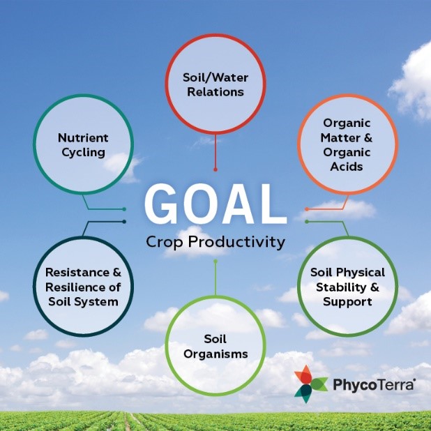
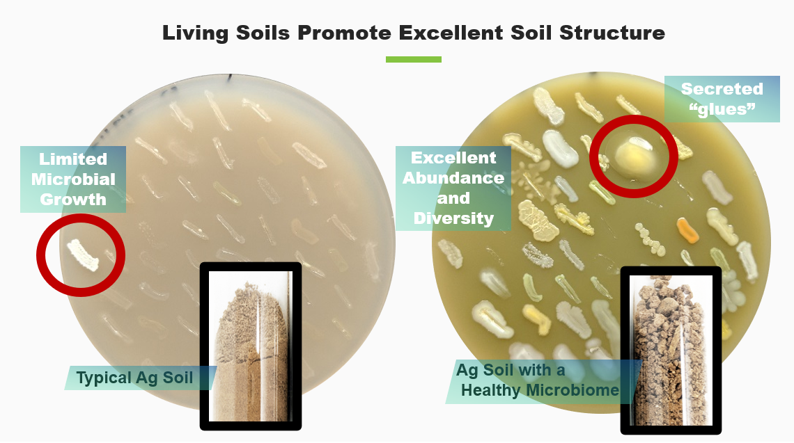
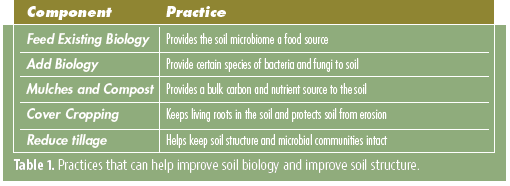

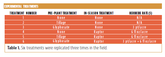

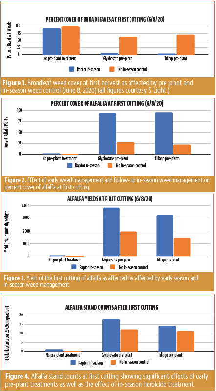


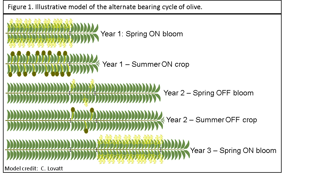
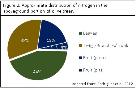
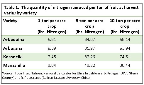

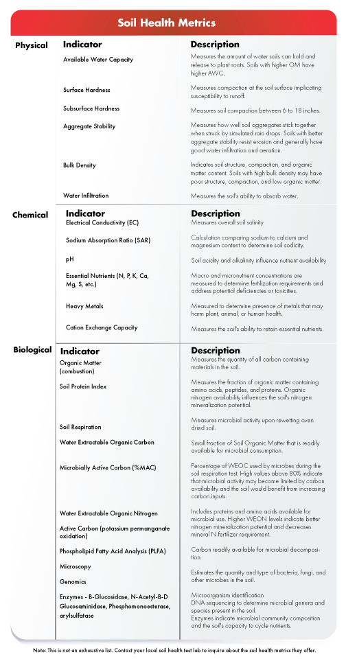

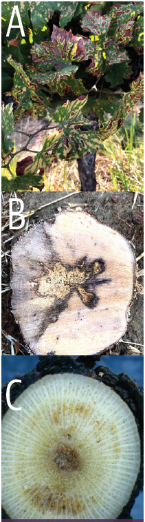
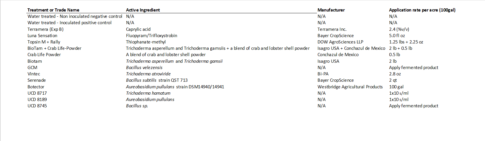
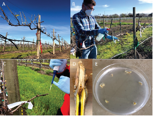
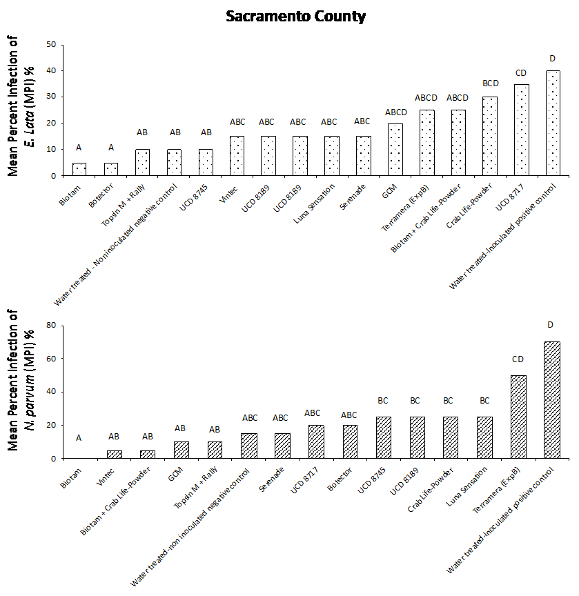
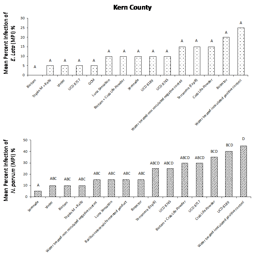


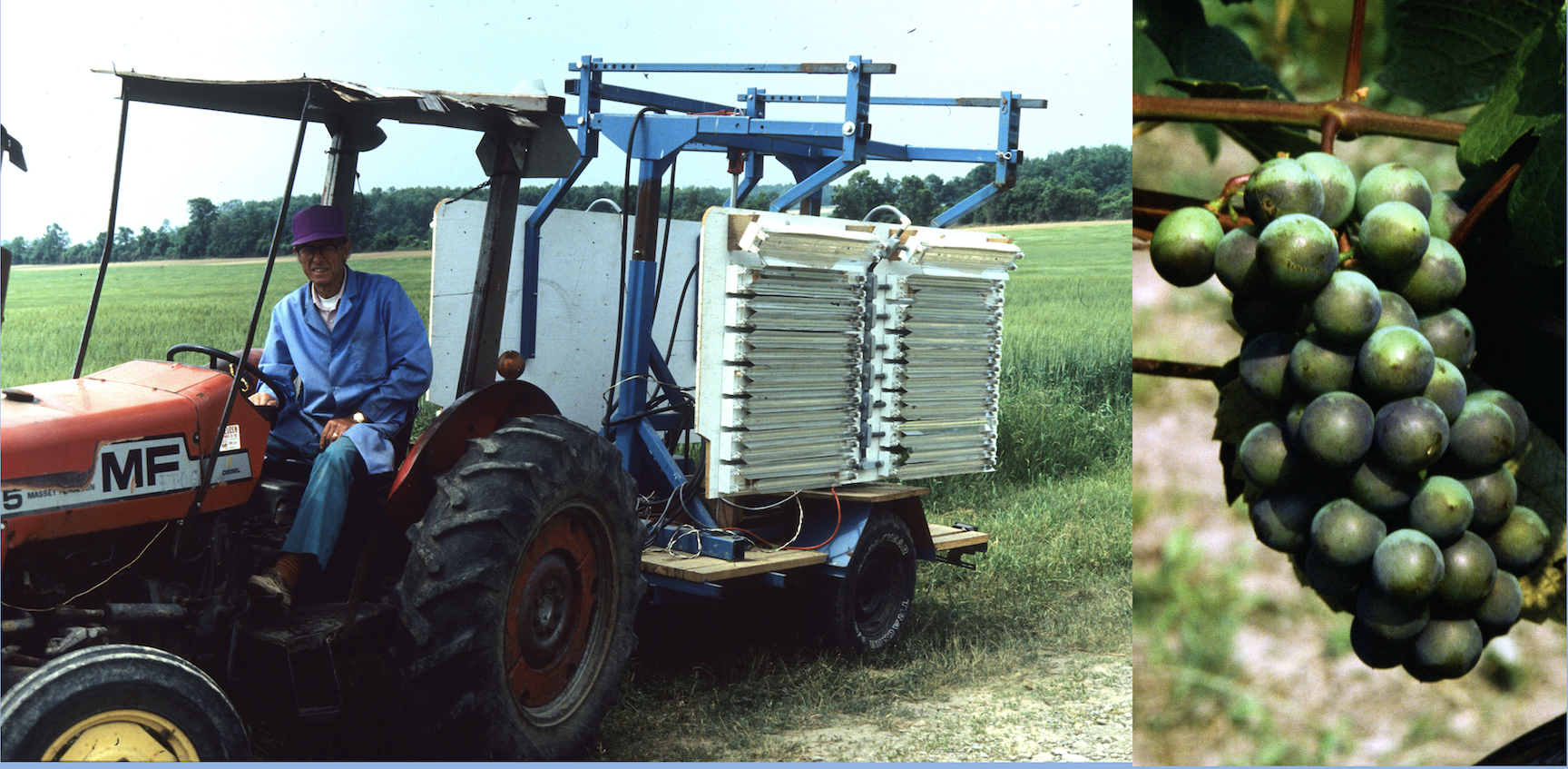
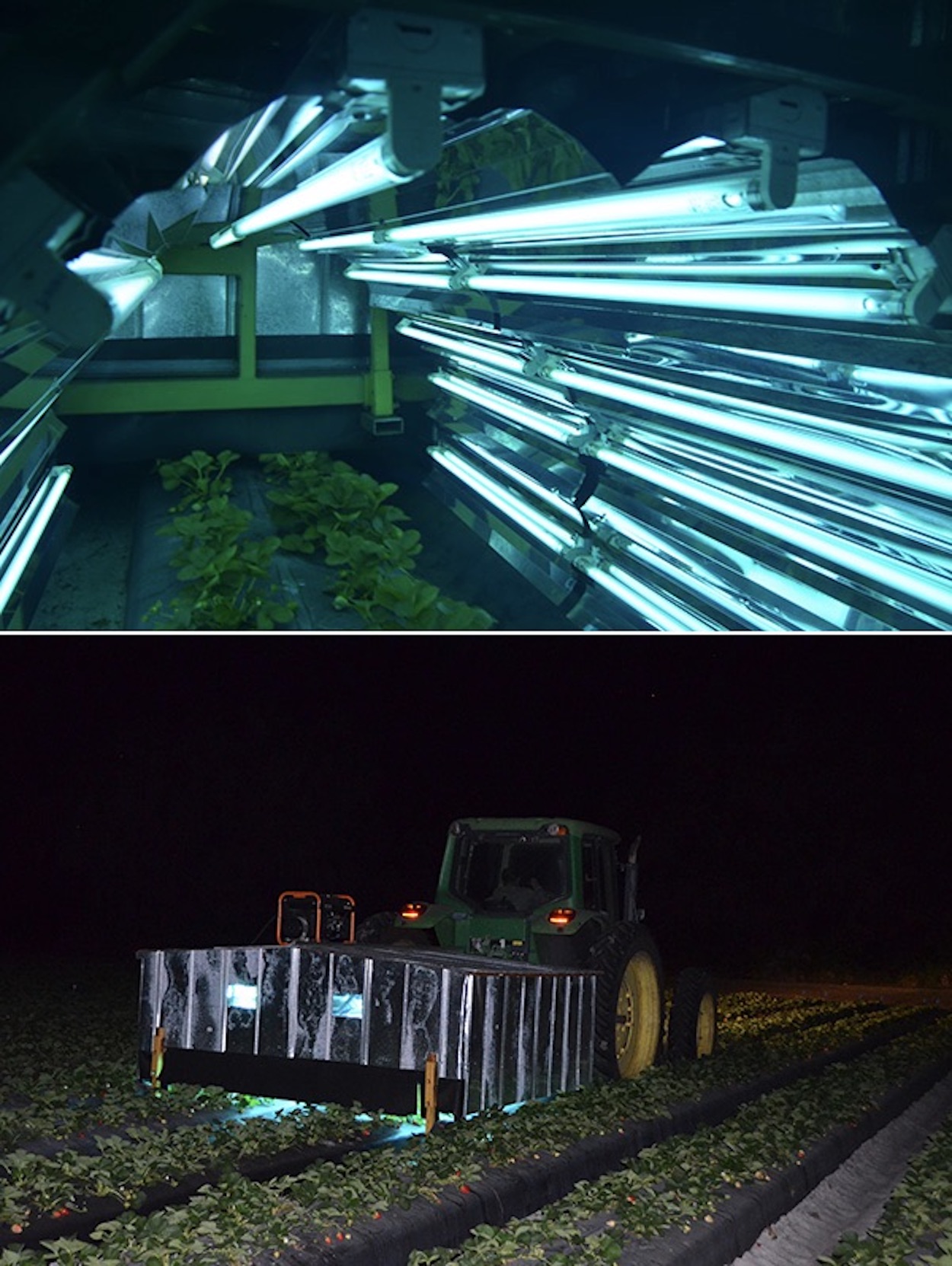
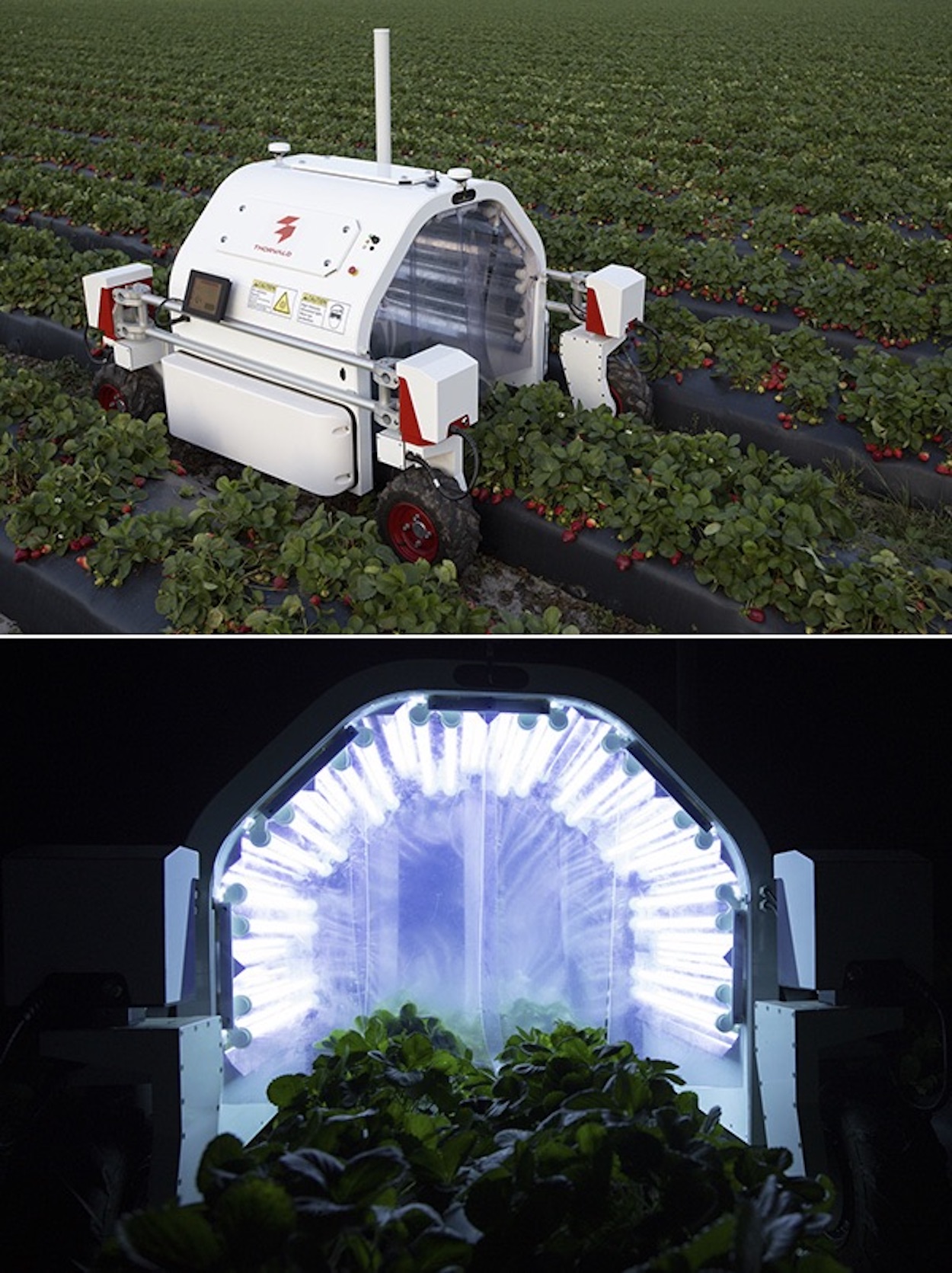
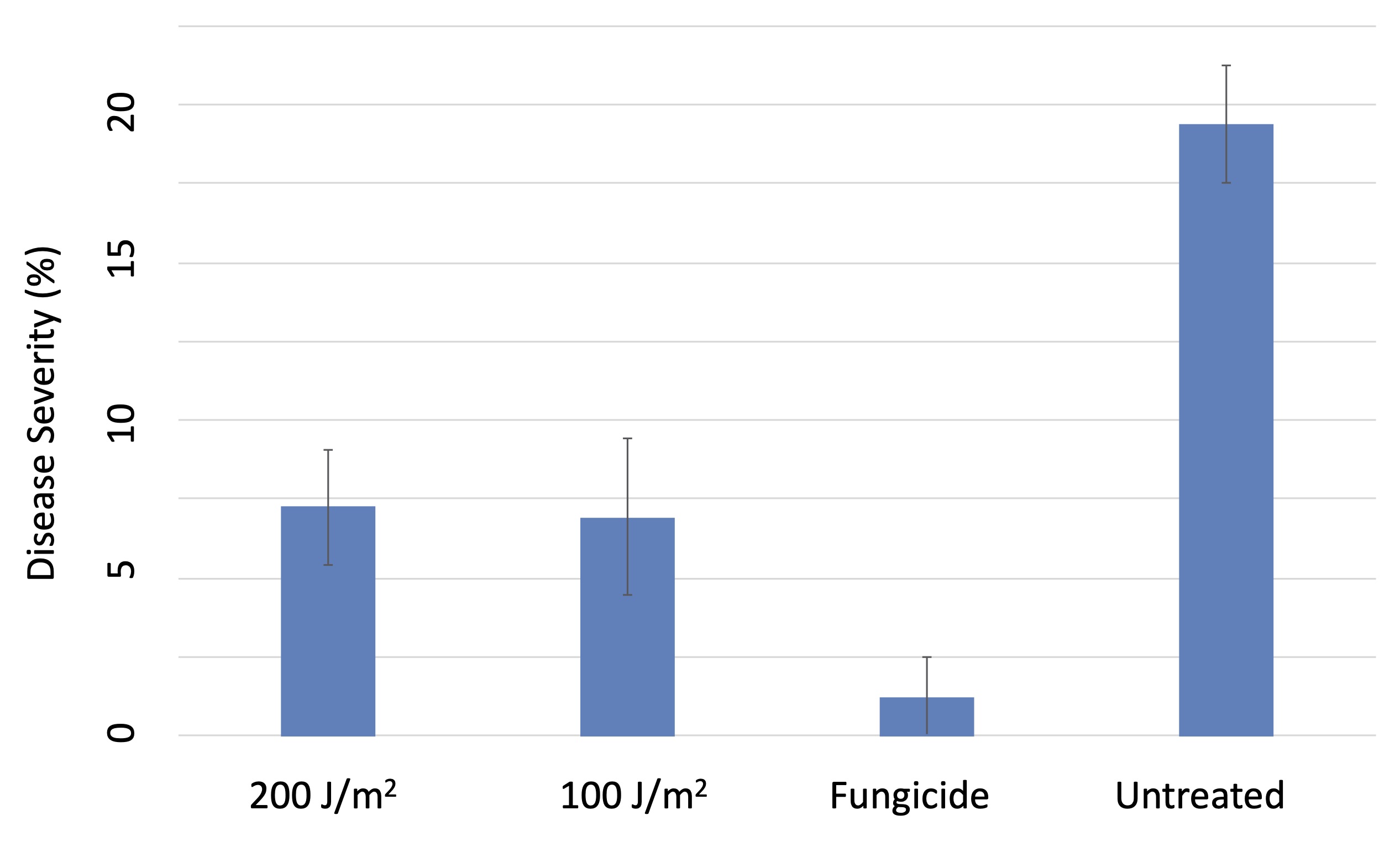
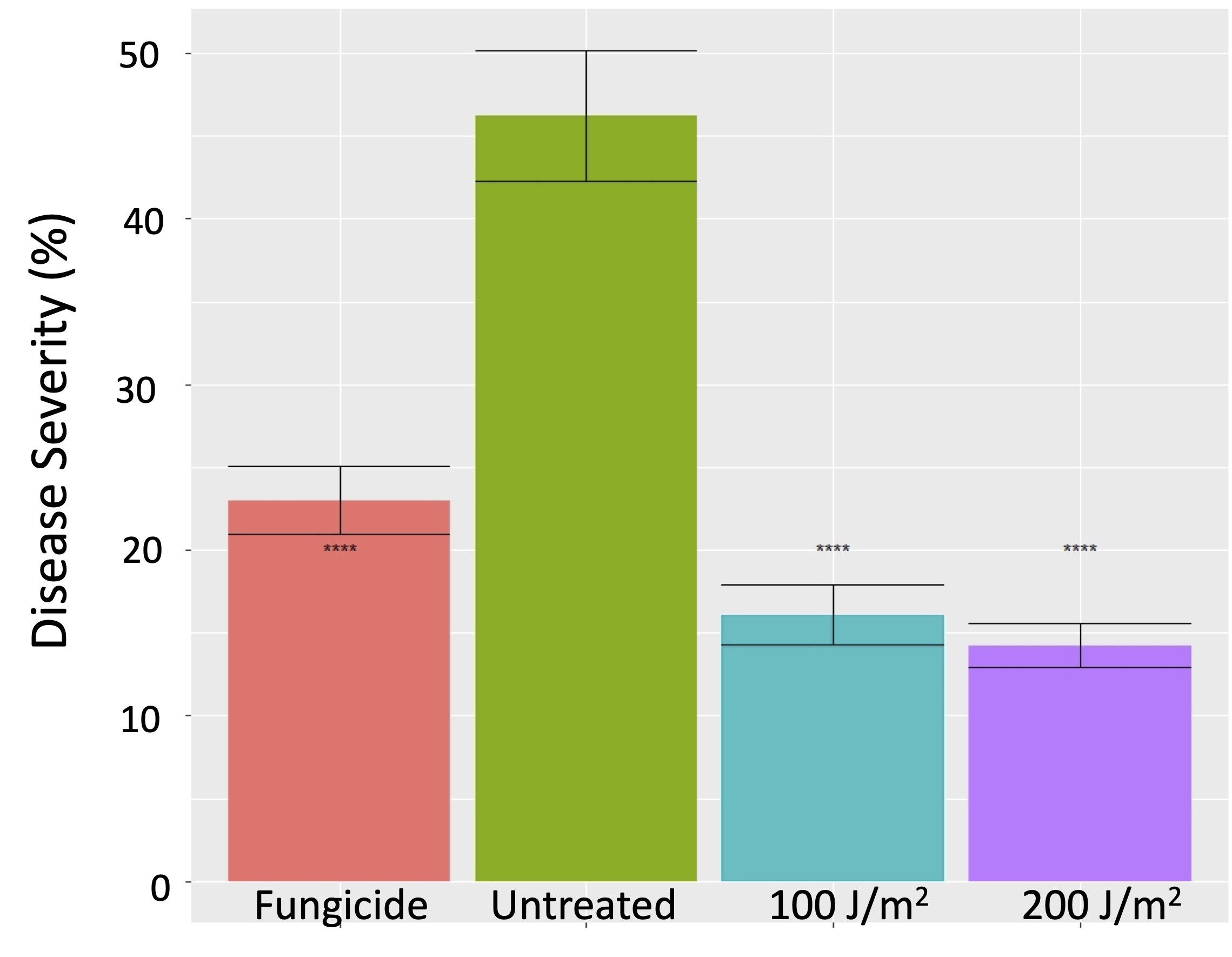

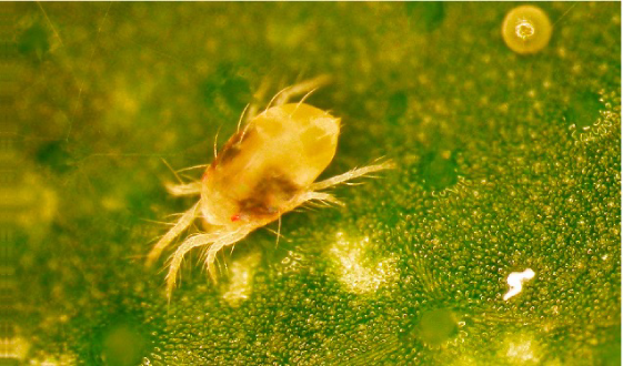
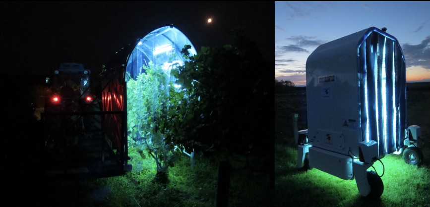
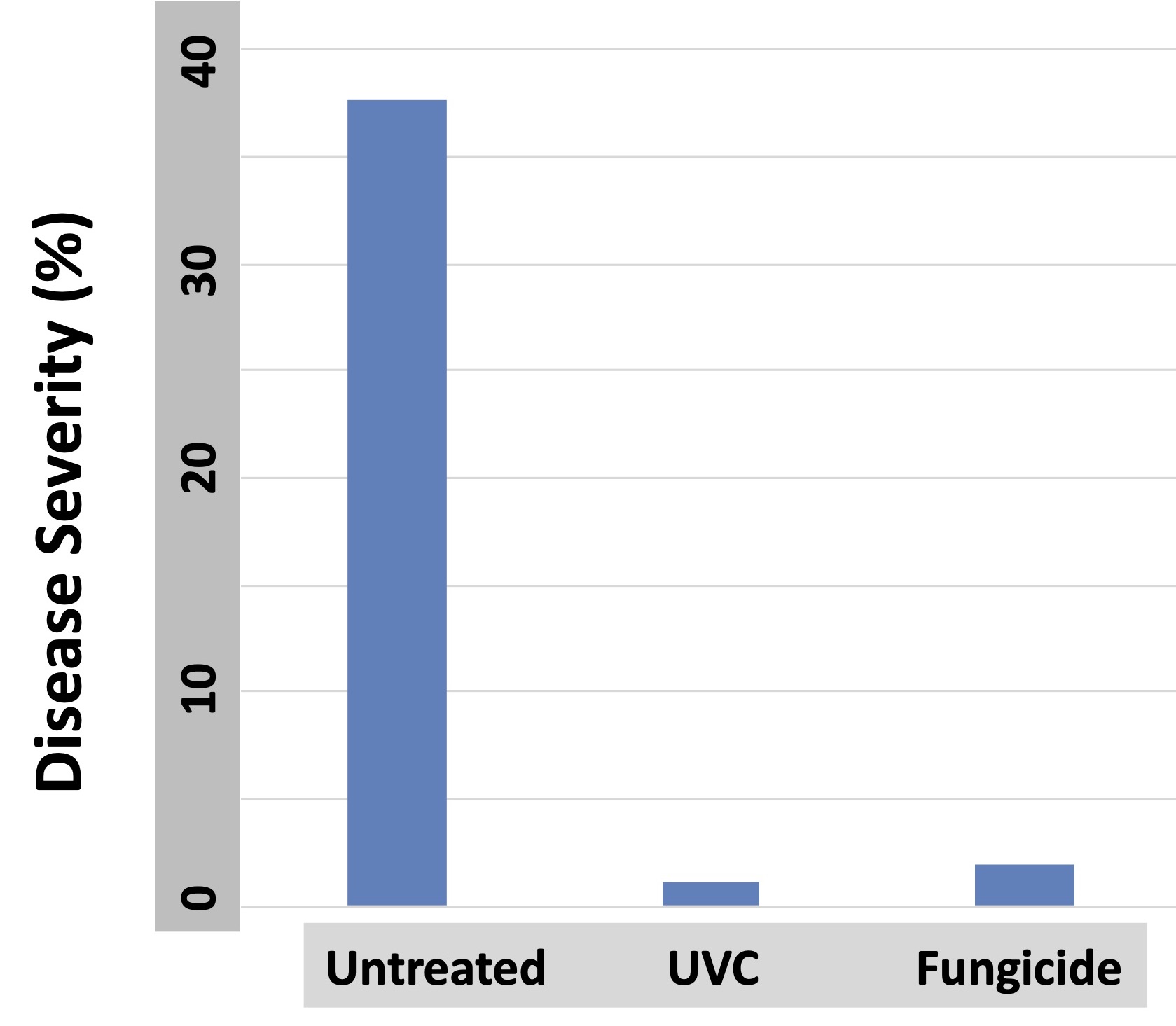


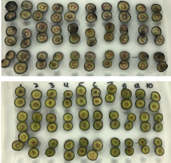
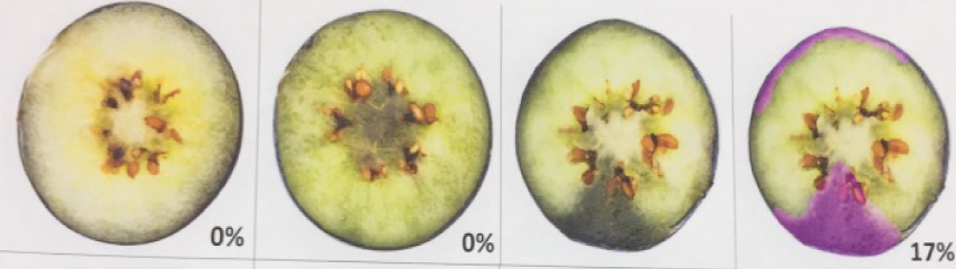
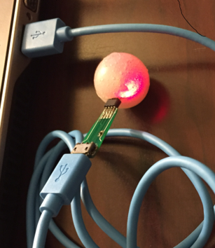
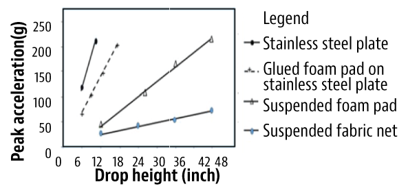
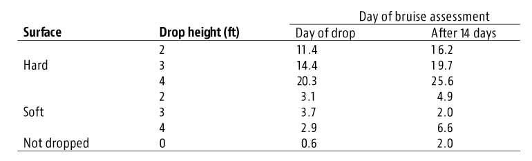
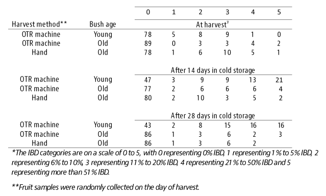
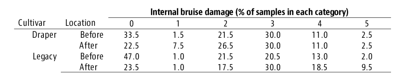


 Invading California")

