
newsletter
Pest Tactic Journal Connects Researchers With Pest Control Industry
Pest Tactic Journal Provides Open-Access Platform for Pest Control Research Pest Tactic Journal was established a few years…
Read ArticleArticle Archive
Pest Tactic Journal Provides Open-Access Platform for Pest Control Research Pest Tactic Journal was established a few years…
Read Article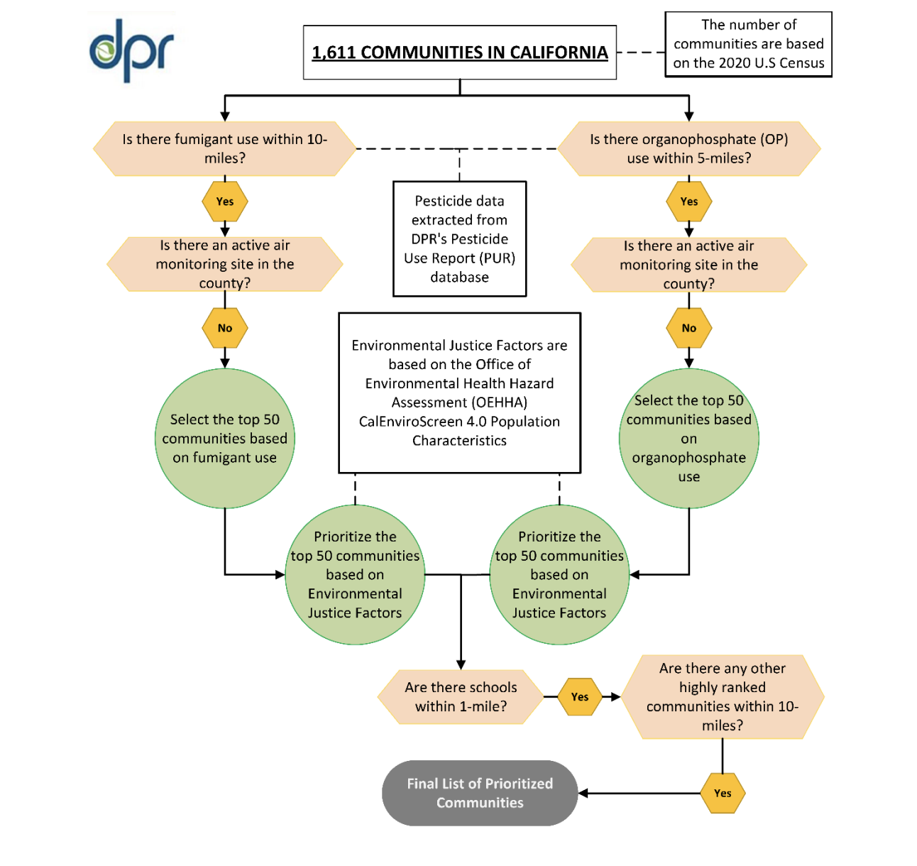
The California Department of Pesticide Regulation (DPR) has announced plans to expand its statewide Air Monitoring Network (AMN).…
Read Article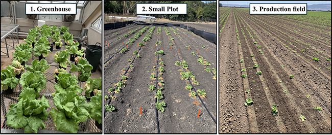
Lettuce Fusarium Wilt Fusarium wilt has become one of the most challenging diseases for California lettuce growers. Once…
Read Article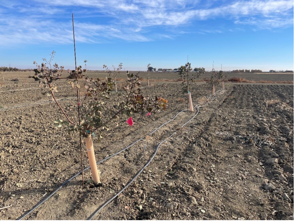
Planting an orchard requires a lot of work to ensure that the trees get off to the best…
Read Article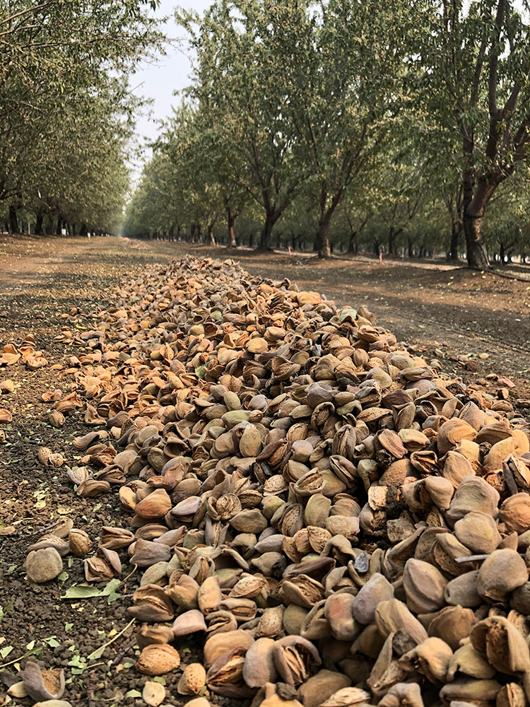
Can almond growers reduce fertilizer application rates without sacrificing yields? That’s the question many are asking as they…
Read Article
Provider of organic and conventional fertilizers will take ownership of global ingredient manufacturer’s botanical-based biopesticides and solutions for…
Read Article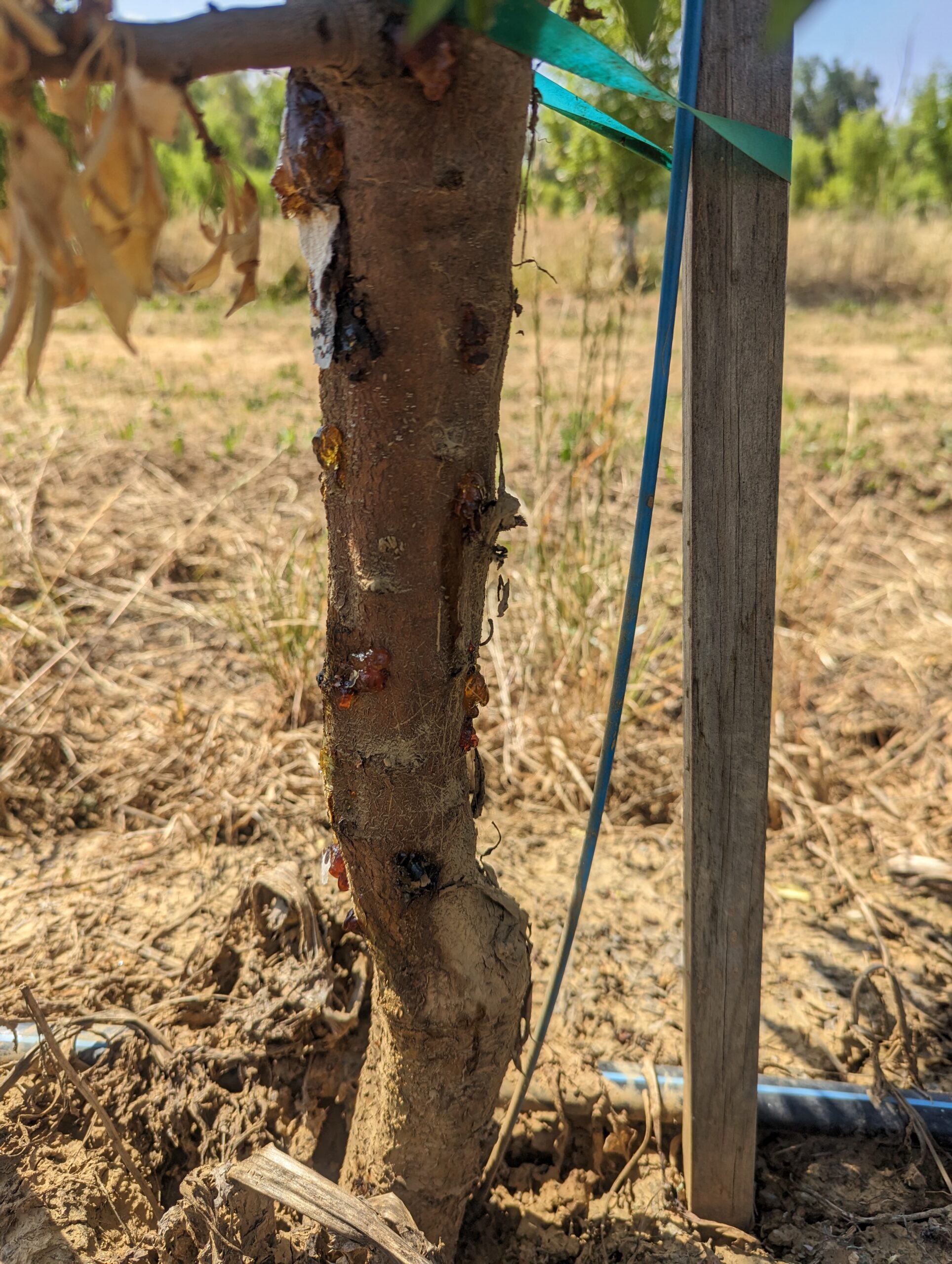
Regardless of your irrigation water source, UCCE farm advisor Jaime Ott emphasizes that irrigation management is Phytophthora management…
Read Article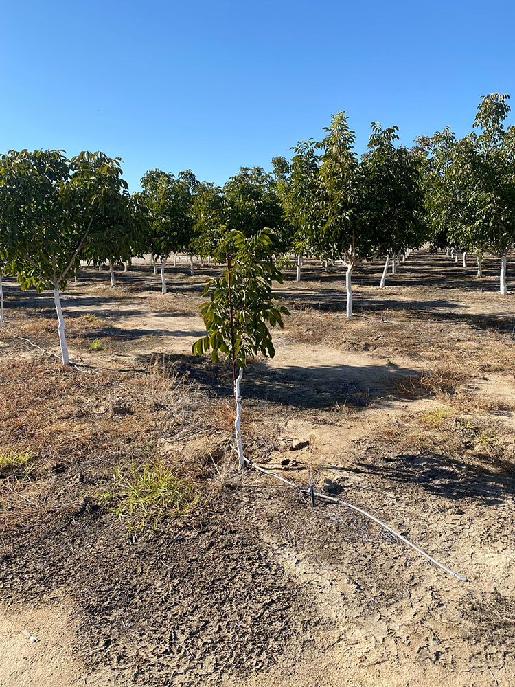
The California walnut industry goes through difficult times. In addition to market challenges, several production issues task the…
Read Article
Visalia, Calif., April 15, 2026 – Sym-Agro announces that Adam Cholakian has joined the company as Southern California…
Read Article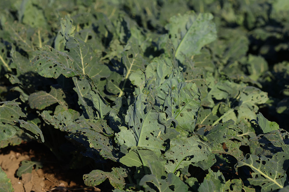
For pest control advisors working in vegetable crops, few insects inspire as much frustration as diamondback moth (Plutella…
Read Article