
Pests
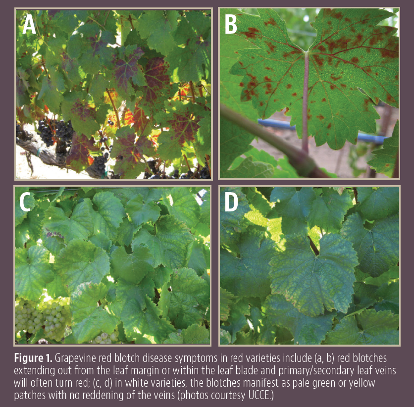
Update on Potential Insect Vectors of Grapevine Red Blotch Virus in California Vineyards
Over the past 10 years, wine grape growers, researchers and UCCE have been working together to control the…
Read ArticleArticle Archive
Over the past 10 years, wine grape growers, researchers and UCCE have been working together to control the…
Read Article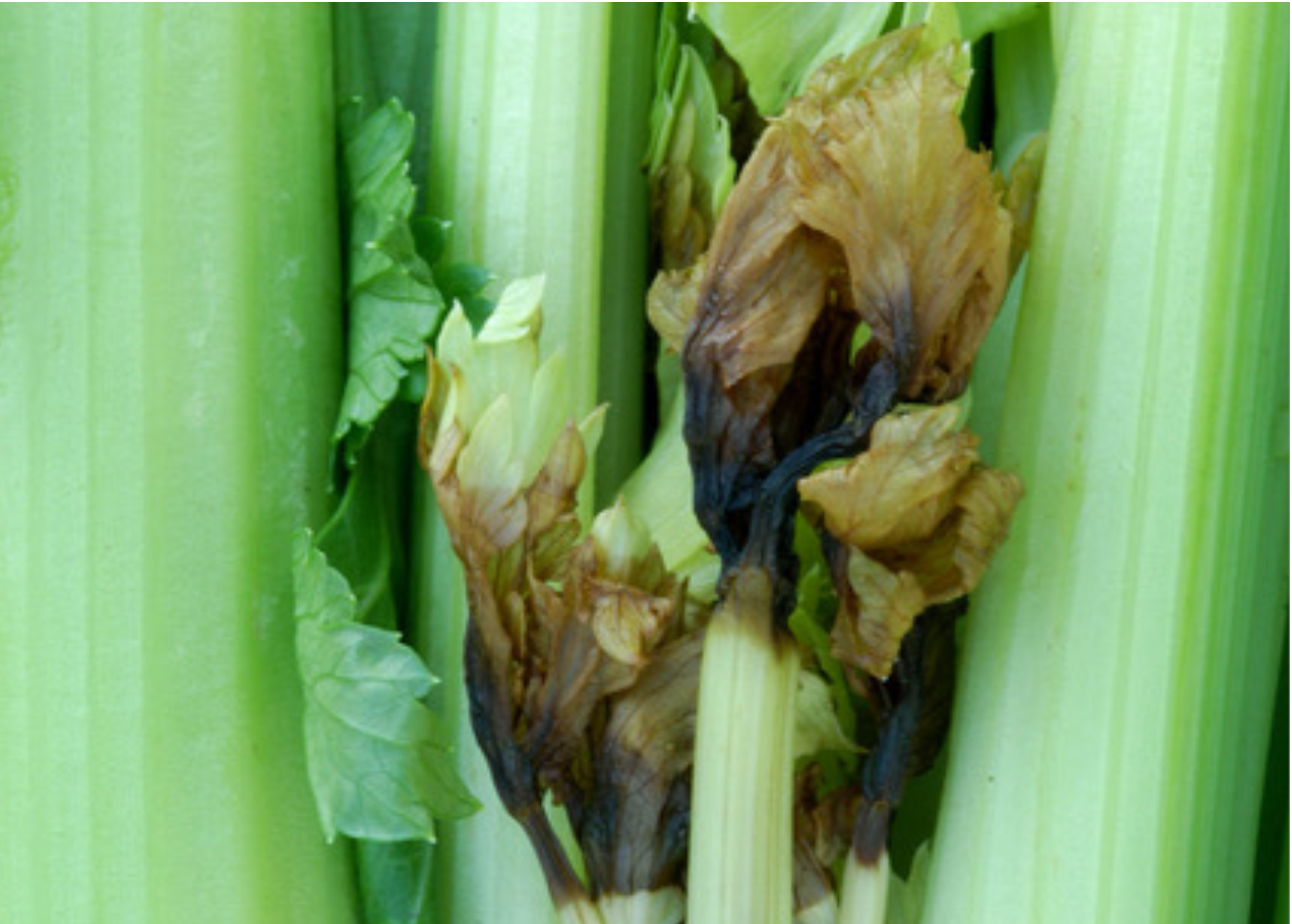
Farmers and agronomists have long observed that well-fed crops tend to suffer fewer pest and disease symptoms compared…
Read Article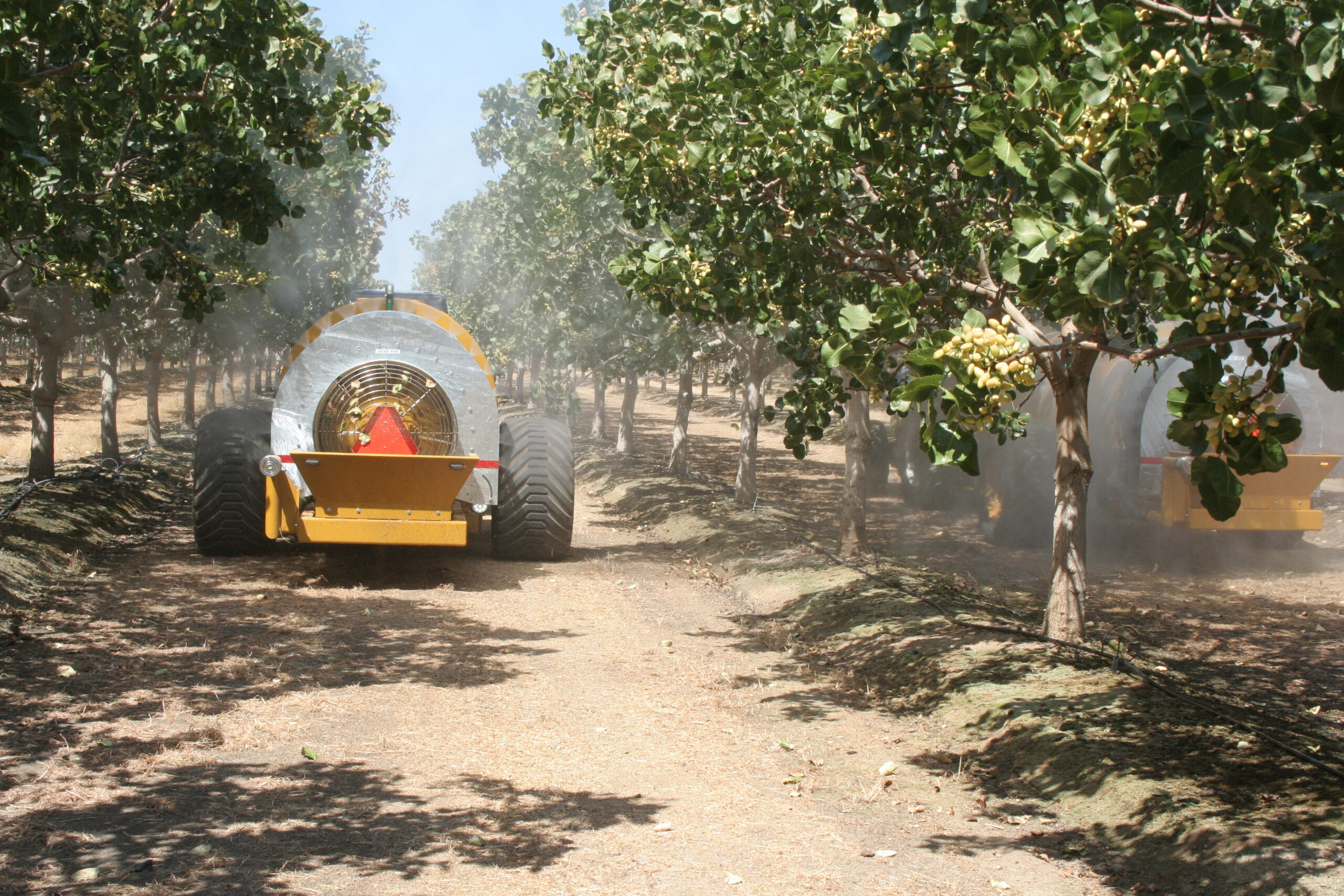
According to studies from the United Nations, the world population will increase by 1 billion people over the…
Read Article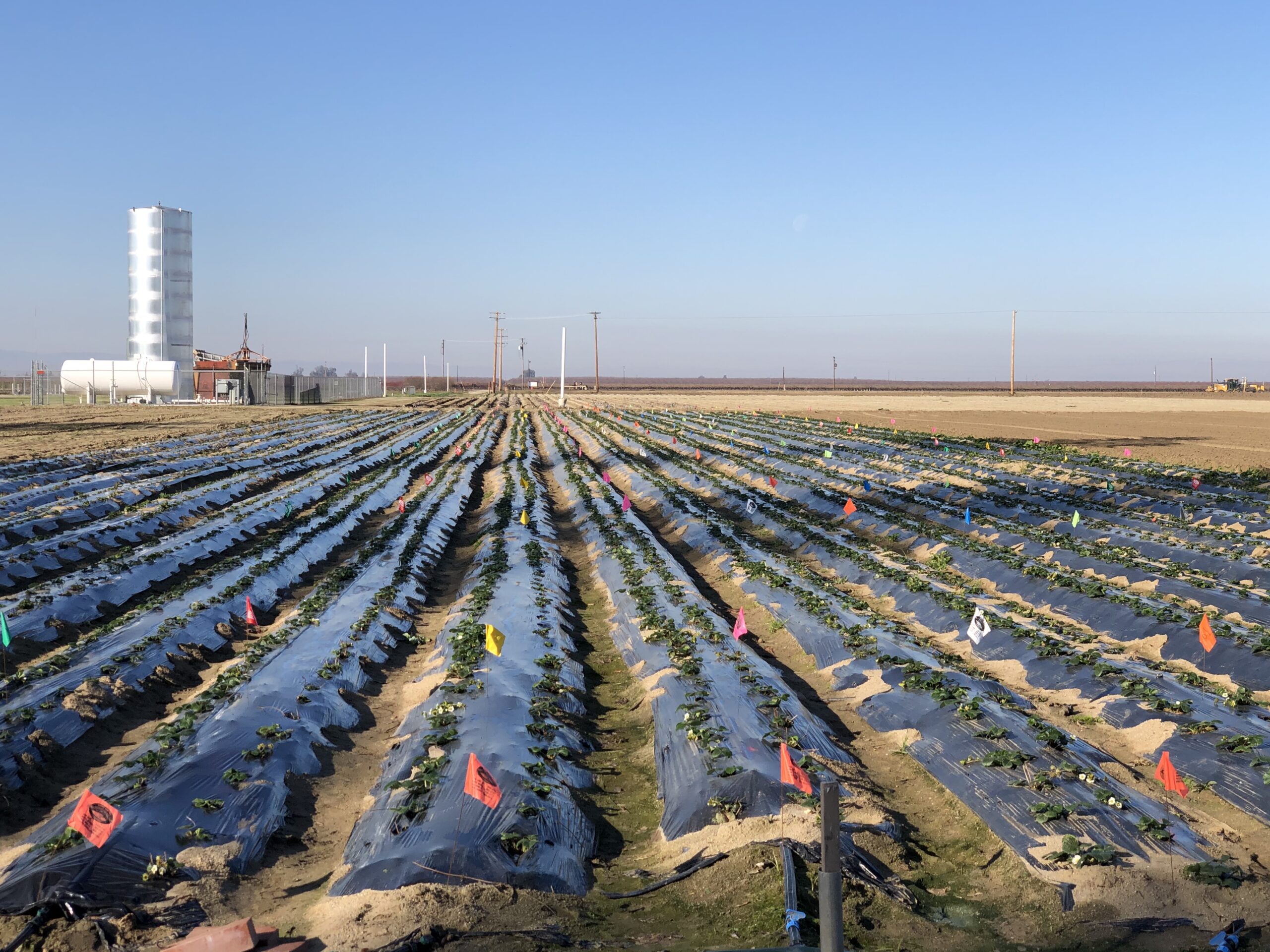
Microbial and botanical biostimulants have been used for promoting plant growth and to help plants withstand various pests,…
Read Article
Soil chemical analysis is the cornerstone of an effective nutrient management program. Without a reliable soil test, significant…
Read Article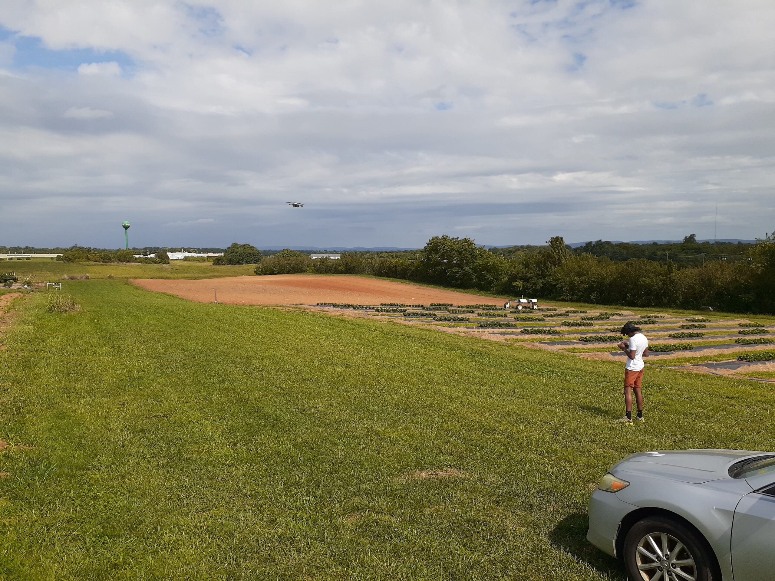
This article summarizes the recent work of a multi-disciplinary research team on strawberry disease and arthropod pest management…
Read Article
Fusarium oxysporum f. sp. lycopersici (Fol) race 3 causes Fusarium wilt, a disease currently affecting most tomato-producing counties…
Read Article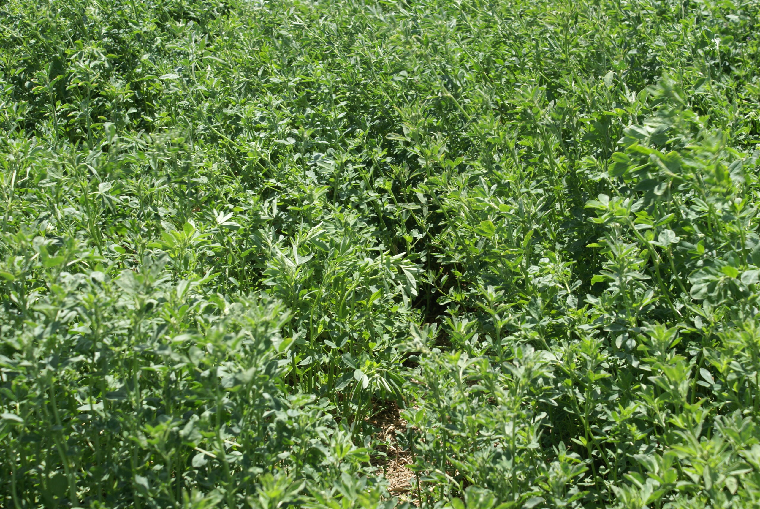
Joint research by UC Davis and UC Cooperative Extension will look at the impact compost applications on young…
Read Article
A robotic pressure chamber that can harvest its own leaf samples and test them on site is being…
Read Article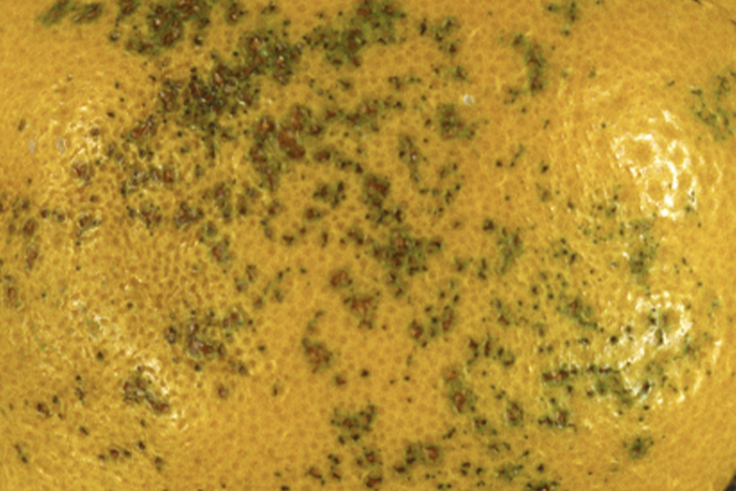
New fungicides that provide a new level of efficacy, along with integrated management practices can help California citrus…
Read Article