


“Soil health” and “healthy soils” have become popular topics in recent years as evidenced by the increased number of government programs and commercial products aimed at improving soil health. The desirable properties of healthy soils are efficiency and efficacy of nutrient cycling, capacity to hold and release plant-available water, an environment conducive to root growth, supportive of beneficial soil organisms and improved resilience of the vine to stress from pests, diseases, drought and/or heat.
Characteristics of a healthy soil are those that promote healthy plant growth:
• A living matrix of plant residues, plant roots, animal residue and microorganisms.
• Porous, with a range of pore sizes that allow a balance between water and air in the soil and space for a complex network of microorganisms (bacteria, fungi, etc.), microarthropods and roots to establish.
• Chemically balanced to allow for nutrient cycling and conducive to the environmental needs of different types of soil organisms in the soil food web and vine roots.
• High in organic matter, which adds nutrients and microbes to soil; those microbes support essential ecological functions of soil, including recycling of nutrients.
Different vineyards and different soil types support different soil ecosystems. What would be considered healthy for sandy soils may not be the same as what is considered healthy for clay soils. Assessing whether the functioning of the soil ecosystem is optimal for any given crop/soil combination is difficult as comparisons between combinations are not necessarily valid.
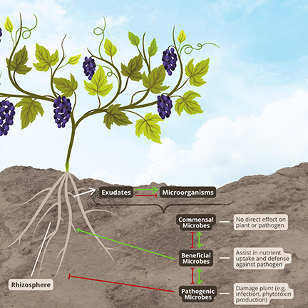
Roles of Microorganisms in Soil Health
Healthy functioning of soil is promoted by complex networks of microorganisms and their grazers, such as beneficial microarthropods. The microbiome of a soil is composed of a host of organisms, including but not limited to bacteria, fungi, protists, nematodes, earthworms and microarthropods. Within these groups, some species can be beneficial, others pathogenic. This can be true even within a genus. For example, the bacteria Pseudomonas fluorescens is beneficial, while Pseudomonas syringae is a pathogen.
Soil microbes play an important role in nutrient cycling in the soil. Decomposers break down organic matter, making it available as an energy and nutrient source for other organisms. Macronutrients such as potassium and phosphorus, which are often immobile in soil, are made available to the vine by some soil microbes.
Soil microorganisms improve soil structure. Bacteria play an important role in aggregate structure and stability. They produce sugars that hold the mineral parts of the soil together. Fungal hyphae weave soils together as do plant roots. Collectively, soil minerals, roots, bacteria and fungi comprise soil aggregates.
Some microbes are biological control agents that antagonize or compete with deleterious microorganisms. For example, predatory nematodes are beneficial. As fungi and bacteria, respectively, Trichoderma spp. and Bacillus subtilis are other examples of well-known biocontrol agents.
Plant growth-promoting bacteria produce chemicals that stimulate vine growth, and amoeba protists stimulate lateral root formation by producing a plant hormone mimic. A vine might react to these compounds like a plant hormone. Other types of bacteria convert nutrients into forms more available to the vine.
Arbuscular mycorrhizal fungi (AMF) live in the soil and on vine roots in a symbiotic relationship with the plant. The plant delivers photosynthates to the fungi for energy, and the fungi provide additional water and nutrients such as phosphorus and nitrogen to the plant. AMF have structures called hyphae that extend great distances through the soil. Hyphae are essentially long tubes that can transport water to vines from areas beyond the root zone. This helps the vine cope with drought. Hyphae also play a role in soil structure.
Soil Microbial Consortia
Soil microbial species do not function in isolation. The survival and success of any one type of soil microorganism is dependent on the presence and activity of many other collaborating microbes. One type of organism provides the resources another type of organism needs or changes the environment such as to favor a different type of organism. Collaborations of multiple species of bacteria and fungi are referred to as a soil microbial consortium. Applying compost to the field can be a method for delivering or manipulating these synergistic soil microbial consortia.
Like other food webs found in nature, soil food webs are composed of multiple trophic levels or positions in the food chain. Communities of organisms perform important ecological functions, such as contributing to plant productivity, decomposing dead and decaying matter, and returning energy and nutrients for use by plants. Numbers decrease as you move from bottom to top, but the biomass per individual increases from bottom to top. Soil food chains may be more complex than aboveground food chains, as they tend to exhibit a greater incidence of omnivory that are capable of foraging on multiple trophic groups.
The three basic pathways that energy is moved between and within trophic levels are roots, bacteria and fungi. Pathogenic fungi, bacteria and nematodes and their consumers comprise the root pathway. The bacterial pathway is made up of bacteria that feed on dead plant material (saprophytic), those that cause diseases in plants (pathogenic), plus the organisms that feed on them, such as protists and bacterial-feeding nematodes.
Fungi found in the fungal pathway include species that are saprophytic, pathogenic and/or mycorrhizal. This pathway also includes consumers of these fungi. Some mesofauna organisms occupy other trophic levels as secondary, tertiary and quaternary predators. Such organisms include protists, nematodes, mites, fly larvae, centipedes, spiders and beetles. The conversion and movement of energy and nutrients around the soil ecosystem is what allows the functions of decomposition, mineralization and soil aggregate formation to occur.
Soils with collaborative suites of microbial species are likely to be more resilient than single species, which are more vulnerable to disease or stress. Species within these communities turn “on” and “off” according to different environmental signals, such that when one classification of soil organisms declines, another one can fill that same role or function. An analogy is an orchestra that features different instruments at different times in a performance. Unfortunately, naming the species composing different soil consortia and their ecological functions in soil health is still in its infancy.
Monitoring Soil Microbiome and Soil Health
Most methods for identifying and quantifying soil microbes are indirect. The methods include measures based on soil aggregation, biomass (estimated by a phospholipid fatty acid profile or counting cells under the microscope), biological activity such as production of extracellular enzymes, and identification by matching DNA fingerprints found in a soil sample to the known genomes of species of bacteria, fungi, protists or nematodes.
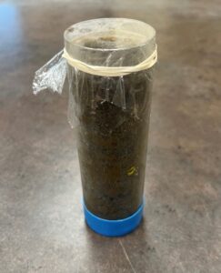
Aggregate stability can be a good measure of soil health because it reflects both physical structure and biology. The bulk density of soil is not a direct measure of soil aggregates but is related. A qualitative way of judging aggregate stability is to take a small sample of soil and drip water on it. If the soil crumbles and falls apart, that is an indication of poor aggregation. If the sample absorbs the water, that is a sign the soil has good structure and ability to hold water. Even if all the species of microorganisms in a soil are unknown, measuring aggregates comprised of bacteria and fungi is useful for monitoring changes through time.
Knowing the functional activity of fungi and bacteria provides a general description of the soil ecosystem and soil health. Functional activity can be measured as enzymes metabolizing specific substrates in soils containing cellulose, amino acids or phosphorus, for example.
Monitoring these and other variables can inform decisions about ground cover, cultivation and fertilization toward the goals of reducing compaction, improving soil aggregate stability, increased water infiltration and disease suppression. The limitation of this type of description is that it does not identify or differentiate what genera or species of these organisms are present. The diversity and complexity of the soil microbiome is crucial to the healthy function of the soil.
Biological Indicators
Soil ecology is the study of the complex interactions between the environment and myriad soil biota. No single measure can capture all the variables that contribute to soil health, but choosing measurements that complement each other can help. Interpreting simple measurements of broad groups like fungi or bacteria is difficult because it does not distinguish pathogens from beneficials.
The biomass of bacteria and fungi can be estimated. Phospholipid fatty acid profiles or cell counts are two methods for estimating microbial biomass. Use of viability stains can distinguish active from dormant organisms. Measuring the ratios between fungi and bacteria can be useful as well because it reflects disturbance. A well-functioning vineyard soil will have a higher ratio of fungi to bacteria, which is promoted by reducing or eliminating tillage to keep vegetation with living roots in the system and avoiding the disruption of the physical characteristics of the microbial habitat.
Measuring respiration in the soil provides a picture of how much life there is in the soil, but it is hard to interpret because it combines respiration of roots, microorganisms and their consumers. Although these measures provide rough estimates of biomass, they do not reflect “who” is there.
Soil organic matter is composed of both living and decaying material. The active or living portion of total soil organic matter can be quantified using a technique based on changes in the color of a potassium permanganate solution mixed with soil. Measurements using this method correlate positively with soil biological activity and are sensitive to management practices.
Current research is being performed to identify sentinel species of microorganisms. If there are genetic markers for these organisms, then identifying specific soil microorganisms is possible. For example, DNA can be extracted from soil. Strands of DNA are replicated using polymerase chain reaction techniques. Those strands are compared to the known genomes of different organisms. The longer the strand of DNA replicated determines how specific identification can be. As the genomes of more soil microbes are mapped, identifying the composition of the microbial community in the soil will become more accurate and useful. This research is still in its infancy.
Encouraging and Conserving Soil Microbial Ecosystem
Diversity of plants in the vineyard increases the diversity of the soil microbial community. This can be achieved with cover crops and grazing. Planting a blend of multiple species of grasses and legumes accomplishes this. Soil covered with vegetation is typically healthier than bare ground.
Applying compost is an excellent way of introducing more carbon into the soil. Compost can potentially inoculate soil with beneficial microbes, provide nitrogen in organic forms and increase soil organic matter overall. The carbon and nitrogen provided by compost feeds both vines and soil microorganisms.
Reducing tillage as much as possible is advisable. Excessive tillage disrupts the soil food web. The mechanical action of tilling severs earthworms and breaks up soil aggregates, which are habitat for beneficial soil bacteria. Hyphae of AMF are torn. Soil organic matter is lost to the atmosphere from tillage, reducing the food source and habitat of many soil microbes. Microorganisms are redistributed in space, separating them from their habitats and food sources such as predators from prey, decomposers from material that needs decomposing, and beneficial relationships between microbes and roots. Organisms surviving a tillage event will need to repopulate and recreate communities within the soil.
Conserving and encouraging the microbial community of the soil is crucial to improving and maintaining soil health. Differences between soil types and the necessities of vineyard management make comparisons difficult. Developing a soil health management program for any vineyard takes time, dedication and the willingness to experiment. Appreciating the role of the soil microbial ecosystems will contribute to the success of a grower’s efforts in improving and maintaining a healthy soil.

")


 Invading California")

