Staying on top of continuing education doesn’t have to mean chasing credits across multiple meetings. The 2026 Crop Consultant Conference is designed to simplify the process, giving PCAs and CCAs a high-value, efficient way to meet CE requirements without losing valuable time in the field.
Instead of piecing together hours from scattered events, attendees can earn a significant portion of their credits in one focused, well-organized conference. Every registration includes access to a free CE tracker to help you log, organize and monitor your hours throughout the year. No spreadsheets. No lost certificates. No last-minute stress.
This event is built specifically for working crop consultants. Sessions are selected for their practical value, with content focused on agronomy, pest and disease management, crop nutrition, regulatory changes and the challenges you face in the field every day. There are no filler topics. Every presentation is chosen for its relevance and direct application, so you leave with tools and insights you can use immediately.
‘The most successful consultants don’t just meet CE requirements. They treat continuing education as part of their professional strategy.’
For busy consultants, the time savings are significant. One event replaces multiple smaller ones. That means fewer days away from growers, fewer miles on the truck and less disruption during a critical time of year. At around $350, the cost compares favorably to what you might spend attending several separate meetings.
Beyond compliance, the conference helps consultants stay ahead of fast-moving changes in labels, regulations and industry practices. That knowledge not only strengthens your recommendations, it reinforces your credibility with growers who rely on you for clear, informed guidance.
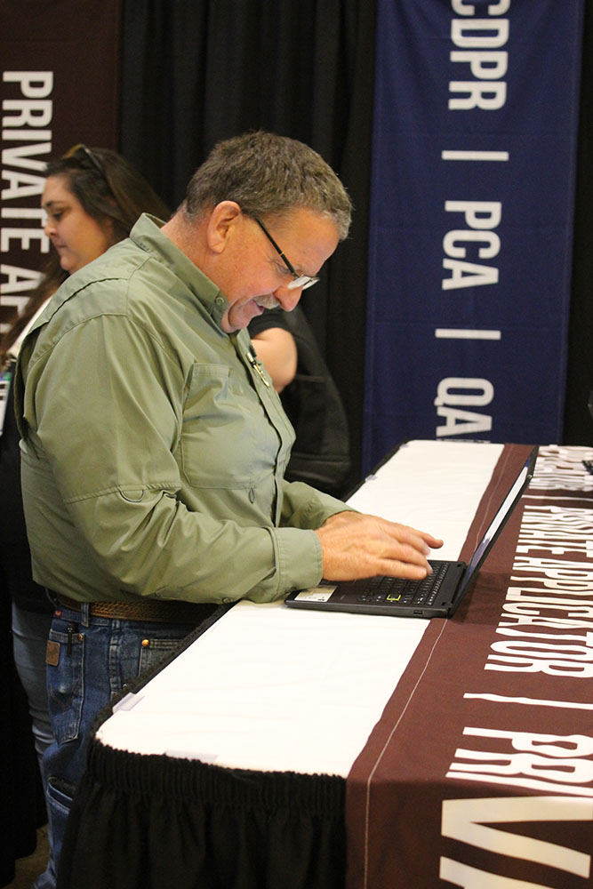
Attendees register at the 2025 Crop Consultant Conference. The event offers a streamlined way for PCAs and CCAs to earn and track continuing education hours in one place. (Photos K. Platts)
There’s also value in being in the room with other PCAs and CCAs. These shared spaces allow consultants to hear what is working, what is not and what new issues are emerging across crops and regions. Those conversations, formal and informal, often prove as valuable as the sessions themselves.
Planning early removes the year-end scramble. You walk away knowing your education is handled and your hours are tracked. That kind of peace of mind is a real asset during a demanding season.
The most successful consultants don’t just meet CE requirements. They treat continuing education as part of their professional strategy. If you want fewer headaches and more value from your CE time, the Crop Consultant Conference, taking place September 23-24, 2026 in Visalia, belongs on your calendar. Register now at https://myaglife.com/crop-consultant-conference/
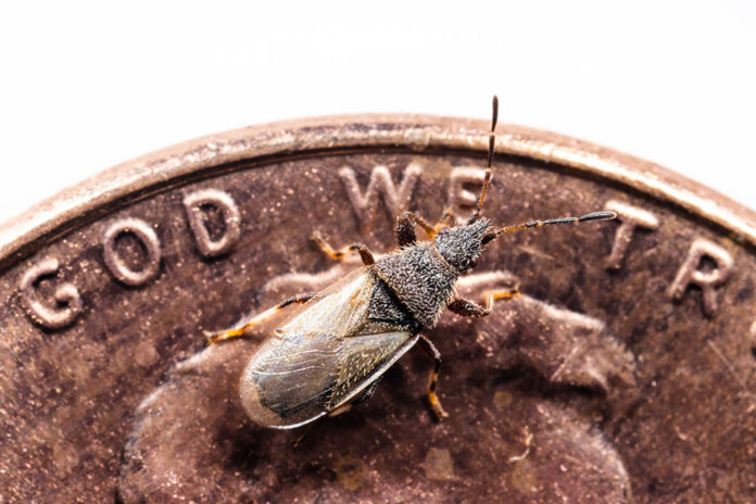
An adult cotton seed bug. (Photo M. Lewis, UC Riverside.)
Cotton seed bug, or CSB, (Oxycarenus hyalinipennis, Hemiptera: Oxycarenidae), is a small seed-feeding bug that poses a significant invasive threat to cotton and other malvaceous crops, such as okra. It is generally regarded as being native to Africa and adjacent Mediterranean regions, from where it has spread widely through trade. From this native range, CSB has successfully invaded parts of Asia, the Middle East, Europe, South America and numerous Caribbean islands. In the early 1990s, CSB established in the Caribbean and was detected in the Florida Keys in 2010. An eradication program targeting this pest in Florida was successfully completed in 2014. The species is well adapted to warm climates and is considered a high-risk pest for U.S. cotton-growing regions in plant hardiness zones 8 to 11.
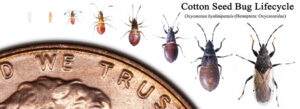
Cotton seed bug has an egg stage (newly laid eggs are white and mature eggs have a reddish hue) five nymphal instars, and adult males and females have a 50:50 sex ratio. (Photo M. Lewis, UC Riverside.)
Host range and biology
CSB is primarily associated with plants in the order Malvales, especially those in the family Malvaceae. Complete nymphal development to adulthood is primarily supported on seeds of malvaceous hosts. Adult CSB, and possibly nymphs, to a lesser extent, may opportunistically use nonhost plants for shelter and moisture sources. Major reproductive hosts include upland cotton (Gossypium hirsutum), okra (Abelmoschus esculentus), various Hibiscus species, kenaf (Hibiscus cannabinus), cocoa (Theobroma cacao) and weedy mallows such as Malva and Abutilon species.
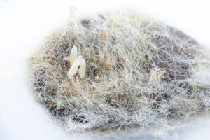
Cotton seed bug eggs freshly laid on lint covering a cotton seed. (Photo M. Lewis, UC Riverside.)
In California, CSB has also been recorded on ornamental Lagunaria species (Norfolk Island hibiscus or cow itch plant) and on seeds of native mallows, such as Abutilon palmeri (Indian mallow), Sphaeralcea species (globe mallow), and Malacothamnus fasciculatus (chaparral mallow), raising conservation concerns for native California mallows. Adults and nymphs aggregate on and inside maturing seed pods of host plants. In cotton, clusters (sometimes referred to as “swarms”) of CSB can be found inside bolls. CSB feeds by inserting needlelike stylets into seeds to ingest endosperm and embryo tissue. Eggs are typically laid in the lint around cotton seeds or inside seed pods of other host plants.
Development from egg through five nymphal instars to adult can be completed in about a month under favorable temperatures, such as 27 C (80 F). Several generations per year, possibly three to seven, may occur on suitable host seeds and favorable temperatures.
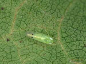
Cotton jassid is a new invasive pest threat to the U.S. cotton industry. (Photo I. Esquivel, Univ. of Florida.)
Economic impacts on cotton
Globally, CSB is considered a major pest of cotton, reducing yield and quality of lint and seed. CSB feeding on cotton seeds can reduce seed weight by approximately 15%. Seed germination rates can also drop significantly, in some cases by up to 88%, which reduces stand establishment success. Additional economic losses may result from lower oil content and quality in cottonseed used for oil extraction. Fiber quality and market grade can be downgraded if lint is stained with fecal spots or reddish fluids released from crushed insects during ginning. The presence of CSB in seed lots may jeopardize market access, adding an indirect but serious economic risk for producers.
Invasion status and risk to California cotton
In California, CSB was first detected in 2019 on Abutilon palmeri in a residential area of Los Angeles County. The California Department of Food and Agriculture (CDFA) has given CSB an “A” rating, defined as an organism of known economic importance subject to quarantine regulation, exclusion, eradication, containment or other holding actions.
‘Globally, CSB is considered a major pest of cotton, reducing yield and quality of lint and seed.’
By 2021–22, subsequent CDFA-confirmed detections in urban areas indicated establishment in Orange, Riverside and San Diego counties. Genetic analyses have supported these findings. There are also credible reports, through personal communications and iNaturalist posts, of CSB in San Bernardino, Ventura, Santa Barbara and Santa Clara counties. However, CSB is sometimes confused with the false chinch bug (Nysius species, Hemiptera: Lygaeidae). Both are small, aggregate-forming bugs. False chinch bugs are generally grayish brown, while CSB is black with a reddish abdomen. Their host plants differ: false chinch bugs favor cruciferous weeds, such as invasive mustards.
While CSB is established in some urban areas, it has not yet been detected in commercial cotton fields, despite targeted surveys by CDFA in major cotton-producing counties in the Central Valley, including Fresno, Kern, Kings, Merced and Tulare. However, proximity to cotton acreage, especially in Riverside County, makes the threat credible. Confirmed detections in San Diego nurseries in September 2025 increase the risk of long-distance accidental introductions to new areas. No other U.S. states have reported CSB to date.
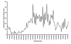
Population phenology of cotton seed bug adults infesting pods of Lagunaria sp. pods on the UC Riverside campus. (Image courtesy UC Riverside.)
Population dynamics in Southern California
Little is known about the population dynamics of CSB in California. Biweekly surveys of Lagunaria seed pods on the UC Riverside campus indicate adult CSB densities increase from October through December, remain steady through March, and decline from April to September before rising again in October.
Natural enemies have been surveyed, with limited findings. Generalist predators such as jumping spiders, sac spiders, pirate bugs (Buchananiella continua), green lacewing larvae (Chrysoperla species) and leafhopper assassin bugs (Zelus renardii) were found infrequently. Lab bioassays confirmed that all six predators fed on at least one CSB life stage, and two, jumping spiders and green lacewing larvae, fed on all stages. However, predator populations were consistently low and did not increase in response to CSB density, providing little measurable control.
Insecticide options
Control is challenging due to CSB’s feeding inside seed pods and cotton bolls. The bug also aggregates in protected sites and overwinters in crop and weed debris.
Insecticides that have shown efficacy against CSB nymphs and adults, and are or have been registered for use in cotton, include:
• Avermectins (abamectin)
• Pyrethroids (bifenthrin, deltamethrin, lambda-cyhalothrin)
• Organophosphates (chlorpyrifos, dimethoate, malathion)
• Neonicotinoids (imidacloprid, thiamethoxam, clothianidin)
• Carbamate/IGR mixes (methomyl and diflubenzuron)
• Spinosyns (spinosad)
• Botanicals (neem oil)
Recent lab studies evaluated 13 formulations. Six, including acephate, dinotefuran, flupyradifurone and imidacloprid, showed efficacy. Insecticide programs targeting pests that damage cotton bolls, such as cotton bollworm (Helicoverpa zea), may also help reduce CSB seed exposure, but repeated applications could increase resistance pressure.
Cotton jassid infestations can cause significant damage to upland cotton. (Photo I. Esquivel, Univ. of Florida.)
Resistance development Lab-selected and field populations of CSB show heritable resistance to multiple chemistries, including imidacloprid, fipronil, organophosphates, pyrethroids, spinosad, emamectin benzoate, chlorfenapyr and nitenpyram. Resistance management must include regular susceptibility monitoring, rotation among classes with different modes of action, and judicious insecticide use.
Cultural and sanitation strategies Cultural controls are recommended to reduce overwintering populations. These include destroying crop residues (stalks, bolls and leaves) through tillage or mulching, removing weeds and alternate hosts, and reducing field-edge refuges. Early picking of cotton bolls may limit exposure time. Covering seed bins before ginning can prevent infestation by flying adults and reduce the risk of spreading CSB to new areas.
Cotton jassid: Another emerging threat
Cotton jassid (Amrasca biguttula, Hemiptera: Cicadellidae) is another pest of concern. Widespread in Asia and newly established in Puerto Rico (2023) and Florida (2024), it spread across the southeastern U.S. by 2025. This pest damages upland cotton at densities of 30 or more per leaf and has a broad host range, including peanuts, soybeans, sunflowers, eggplant, potatoes and ornamental hibiscus.
With both cotton seed bug and cotton jassid now in the U.S., it is increasingly likely they will co-occur in production regions. Existing IPM programs will need to be adapted to address these new threats. Localized strategies and strong extension support will be essential for sustainable management.
References
Adachi-Hagimori, Triapitsyn SV, Uesato T. 2020. Egg parasitoids (Hymenoptera: Mymaridae) of Amrasca biguttula (Ishida) (Hemiptera: Cicadellidae) on Okinawa Island, a pest of okra in Japan. Journal of Asia Pacific Entomology 23: 791-796. https://doi.org/10.1016/j.aspen.2020.07.008
Halbert SE, Dobbs T. 2010. Cotton seed bug, Oxycarenus hyalinipennis (Costa): A serious pest of cotton that has become established in the Caribbean Basin. Pest Alert: Florida Department of Agriculture and Consumer Services, Division of Plant Industry. DACS-P- 01726. https://ccmedia.fdacs.gov/content/download/9773/file/oxycarenus-hyalinipennis.pdf (accessed 24 Nov. 2025)
Hoddle, CD and MS Hoddle. 2023. Cotton seed bug: another invasive pest that has established in California. CAPCA Adviser 26(1): 34-38.
Ijaz M, Shad SA. 2018. Inheritance mode and realized heritability of resistance to imidacloprid in Oxycarenus hyalinipennis Costa (Hemiptera: Lygaeidae). Crop Protection 112: 90-95. https://doi.org/10.1016/j.cropro.2018.05.015
Irshad M, Salem MM, ul ain Hanif Q, Nasir M, Asif MU, Shamraiz RM. 2019. Comparative efficacy of different insecticides against dusky cotton bug (Oxycarenus spp.) under field conditions. Journal of Entomology and Zoology Studies 7(2): 125-128.
Texas Department of Agriculture. 2025. Cotton Jassid – Two-Spot Cotton Leafhopper (Amrasca biguttula). https://texasagriculture.gov/Regulatory-Programs/Plant-Quality/Pest-and-Disease-Alerts/Cotton-Jassid-Two-Spot-Cotton-Leafhopper (accessed 4 December 2025).
Ullah S, Shad SA, Abbas N. 2016. Resistance of dusky cotton bug, Oxycarenus hyalinipennis Costa (Lygaidae [sic]: Hemiptera), to conventional and novel chemistry insecticides. Journal of Economic Entomology 109: 345-351. https://doi.org/10.1093/jee/tov324
USDA-APHIS. 2024. Pest alert: Cotton seed bug (Oxycarenus hyalinipennis). United States Department of Agriculture, Animal and Plant Health Inspection Service, Plant Protection and Quarantine. Available from: https://www.aphis.usda.gov/sites/default/files/alert- cotton-seed-bug.pdf (accessed 25 Nov. 2025)
Wazir S, Shad SA. 2022. Development of fipronil resistance, fitness cost, cross-resistance to other insecticides, stability, and risk assessment in Oxycarenus hyalinipennis (Costa). Science of the Total Environment 803: 150026. https://doi.org/10.1016/j.scitotenv.2021.150026
Zilnik, G, JR Hepler, P Merten, IX Schutze, CD Hoddle, MS Hoddle, PC Ellsworth, and C Brent. 2025. Screening of insecticides for management of the invasive Oxycarenus hyalinipennis Costa (Hemiptera: Oxycarenidae) population sourced from urban southern California. Journal of Economic Entomology 118(2): 692-699. https://doi.org/10.1093/jee/toaf014
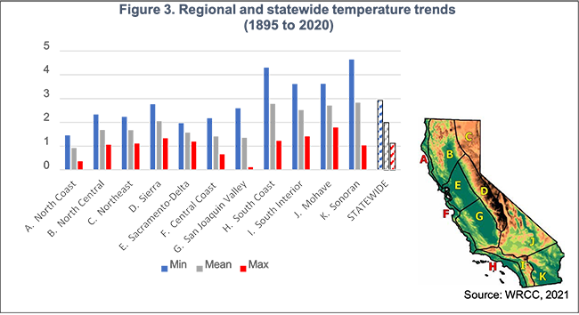
Minimum temperatures are rising faster than maximums, especially in key ag regions like the San Joaquin Valley—affecting crop performance and pest cycles. (Source: WRCC, 2021)
California’s agriculture is a cornerstone of both the state and national economy, generating more than $60 billion in annual farm revenue from a diverse mix of more than 400 commodities and contributing significant export value globally. That production occurs on agricultural landscapes spanning irrigated cropland and extensive rangelands for livestock. Irrigated agriculture, which produces the majority of specialty crops in California, takes place on less than 10 million acres of land, yet the state leads the nation and world in producing several commodities. Despite this leadership position, current and future changes in climate pose a major threat to the state’s agricultural sector.
Farmers, crop consultants and technical service providers are under constant pressure to adjust and adapt to both weather variability and long term climate change. This article outlines how climate has changed in the past and is projected to change in the future, how these stressors are affecting California agriculture and why adaptation is needed to make agriculture more resilient to these risks.
Rising temperatures
Across California, average temperatures have increased significantly. Over the last century, minimum temperatures rose about 3°F and maximum temperatures by a little more than 1°F. Different regions in the state have experienced warming at varying magnitudes, but in general the increase in minimum temperatures has been greater than that for maximum temperatures. Future projections indicate that temperatures will continue rising throughout the 21st century. By mid century, average temperatures are expected to increase by approximately 2.5°F to 3.5°F under moderate emissions scenarios and 4.5°F to 5.6°F or more under high emissions scenarios, relative to late 20th century conditions.
‘Most farmers reported experiencing greater climate impacts on their farms compared to a decade ago, reflecting lived experience rather than abstract awareness.’
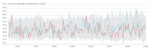
Changes in precipitation and water availability Climate change is altering not just total precipitation, but also its timing and form. Reduced snowpack and earlier runoff are placing increasing pressure on surface water supplies and groundwater. Current long term data do not show a consistent statewide trend in total annual precipitation, but increased variability and extremes are expected. This means prolonged droughts as well as more intense storms and flood conditions may become more common. Because nearly all specialty crops in California are irrigated, uncertainty in precipitation and water availability is a critically important issue for agriculture.
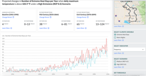
Increasing frequency and intensity of extreme heat The increasing frequency and intensity of extreme heat is among the most concerning climate threats facing California agriculture. Extreme heat is commonly defined using locally relevant temperature thresholds, such as days when maximum temperatures exceed 95°F or 100°F, or when nighttime minimum temperatures remain high. These thresholds are typically based on the upper percentiles of long term temperature records. Future trends show a substantial increase in the number of days exceeding these heat thresholds, with the most significant increases projected for inland valleys, desert regions and urbanized areas. By midto late century, many parts of the Central Valley and Southern California are expected to experience several dozen additional extreme heat days per year compared with historical conditions. Coastal regions, though moderated by marine influence, are also projected to see more frequent and intense heat events. Extreme heat is spreading both spatially and temporally, regions that historically experienced only occasional heat waves are increasingly exposed, heat seasons are starting earlier and ending later, and nighttime heat extremes are becoming more common. This expanding footprint of extreme heat amplifies risk to agricultural productivity across the state.
Precipitation shows no long term trend but greater extremes, with more intense droughts and wet years expected, heightening irrigation uncertainty.
Farmer perceptions of climate impacts
Farmers have firsthand experience with how climate variability and long term climate change affect their operations. In a statewide survey, researchers observed broad recognition among farmers that climate change is occurring and relevant to agriculture. About two thirds of surveyed farmers agreed that climate change is happening and that actions are necessary to address it. Most farmers reported experiencing greater climate impacts on their farms compared with a decade ago, reflecting lived experience rather than abstract awareness. Perceived impacts were dominated by water related concerns, including reduced and uncertain irrigation water supplies and declining groundwater availability, followed by temperature related stresses such as increased drought severity and extreme heat affecting crops. Disaster risks, including partial or complete crop and farm losses, were also noted. Perceptions varied across regions, crop types and farmer demographics, with historically underrepresented and limited resource farmers generally expressing higher levels of concern. Many growers expressed interest in learning more about climate impacts and adaptation options.
Extreme heat days over 103.9°F could rise from 4 to over 120 per year by 2100 under high emissions, threatening worker safety and crop health. (Source: Cal-Adapt)
Research perspectives on climate impacts
Long term trends show that climate change is already altering California’s agricultural climate in ways that directly affect crop yields and production patterns. Rising average temperatures, more frequent and severe droughts and heat waves, changing precipitation patterns and diminished snowpack all place stress on water intensive cropping systems and limit water availability for irrigation across the state’s diverse farming regions. These shifts disrupt both annual and perennial crop phenology, reducing chill hours for fruit and nut trees and potentially shortening growing seasons, which can lower yields and challenge the viability of high value crops such as grapes, almonds and citrus if adaptation measures are not implemented.
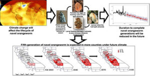
Warming is expected to trigger a fifth navel orangeworm generation in more counties by 2100, increasing crop losses and aflatoxin risk. (Source: Pathak et al. 2021), https://www.sciencedirect.com/science/article/pii/S0048969720361866
Enhanced climate variability also increases the likelihood of extreme events such as floods or prolonged drought, further threatening crop productivity and farm sustainability. Beyond the direct effects on plant growth, climate change is expected to intensify pressures from agricultural pests, which can further depress yields and increase production costs. Research on insect pests affecting California’s high value specialty crops indicates that warmer temperatures will shift the timing of pest life cycles, leading to earlier seasonal emergence and potentially more generations per season. For example, key pests such as codling moth, peach twig borer, oriental fruit moth and navel orange worm are projected to complete additional generations per season under future climate conditions, increasing their cumulative impact on crops like walnuts, almonds and peaches. These changes complicate pest management efforts and could increase reliance on chemical or other interventions, with economic and environmental consequences for growers.
Enhancing agricultural resilience to climate risks The combined effects of climatic stressors and biological responses underscore the need for comprehensive adaptation strategies. Climate change influences multiple factors simultaneously, including water demand, heat stress and pest and disease dynamics, and demands locally tailored responses that integrate improved water management, selection of resilient crop varieties and proactive pest management. Strengthening agricultural adaptive capacity through climate smart and regenerative practices, improving soil health and better integration of climate information into strategic decisions will be essential for maintaining productivity, protecting food security and supporting the economic value of California agriculture in the face of ongoing and future climate challenges.
Crop consultants who integrate climate information into their recommendations will be better positioned to support growers facing expected climate challenges and higher uncertainties. Climate informed consulting is an important component of best management practices to enhance agricultural resilience to climate related threats.
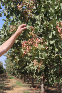
Understanding How Cover Crops Affect Water Use in Pistachio Orchards
If I plant a winter cover crop, will it use water my trees need?
It is a question more growers are asking as interest in soil health practices increases and water uncertainty continues across California. Many growers still wonder what the trade-offs might be, especially in years when every inch of water matters. To move beyond assumptions and gather real field measurements, our team established a multiyear comparison study at Bullseye Farms in the Sacramento Valley to help answer this question. Growers want straightforward answers, but until recently, there were very few field studies directly measuring these trade-offs in commercial pistachio orchards. With pistachio acreage expanding across the Central Valley, these questions are becoming increasingly important for long-term orchard planning.
Inside the Study at Bullseye Farms Our team, including Bullseye Farms, the USDA-ARS Sustainable Agricultural Water Systems Unit, and the University of California, Davis Agricultural Water Center, is studying water use and soil moisture dynamics in two adjacent pistachio orchards, one managed with a winter cover crop (CC) and one maintained without (NC). Both blocks were planted with Golden Hills in the same year, use the same double-drip irrigation system, and sit on similar silt loam soils.
The CC orchard has been growing cover crops since 2019, using a general mix of beans, peas, vetch, grains and brassicas typically planted in early November. Because the orchards are identical in age, variety and irrigation, the only major difference between the two systems is the presence of the cover crop itself, which offers a clean comparison of how cover crops influence soil moisture and evapotranspiration (ET).
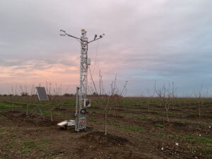
Research installation at the 152-acre orchard began in early 2023. Separate eddy covariance towers were installed in each orchard to directly measure ET. In addition, 36 12-foot neutron probe access tubes were installed at four randomly selected locations in each orchard—72 total—allowing us to monitor soil moisture from the surface down to 10 feet. Installation was completed by September 2023.
This level of instrumentation makes these orchards among the most closely monitored pistachio orchards in California. It allows us to see not just whether cover crops use water, but how they change the timing, depth and distribution of water in the soil profile. Biweekly soil moisture measurements have continued since installation, and we now have two full seasons of data showing how cover crops influence orchard water dynamics.
‘Cover crops may not use water that trees need, but they do change when and where water is stored and used in the orchard.’
What We’ve Seen in Soil Moisture and ET After two seasons of monitoring, a clear and consistent pattern has emerged: cover crops shift both where and when water is stored and used in the soil profile.
In the upper five feet, the CC orchard generally showed lower moisture during the winter and early spring due to active water use by the cover crop.
Deeper in the profile, around five to seven feet, the CC orchard consistently stored more moisture than the NC orchard. This deeper storage is consistent with other studies showing that cover crops can improve infiltration and move water deeper into the soil. For a deep-rooted perennial like pistachio, this water may become important later in the irrigation season, especially in mature orchards where roots extend well below the shallow layers that dry out quickly.
An interesting finding is that the timing of early winter rainfall did not change this pattern. The 2024–25 season received its first rainfall about a month earlier than the 2023–24 season, yet the contrast between shallow drying and deeper storage remained the same. This suggests that the infiltration benefits from the cover crop are not highly sensitive to when the first winter rainfall arrives.
Evapotranspiration (ET) patterns help explain the bigger picture. Over the full November through October monitoring period in 2023–24, total ET differed by only about 1 inch between the two orchards.
The key difference was when that water was used. The CC orchard had higher ET from November through April, driven by winter cover crop growth. Surprisingly, the NC orchard had marginally higher ET from July through October, possibly due to the protective mulch layer left in the CC orchard after termination reducing soil evaporation.
The orchard had its first harvests in 2024 and 2025. Over both seasons, there has not been a significant difference in yield between the two orchards. While it is still early in the orchard’s lifespan, initial signs suggest that the presence of a winter cover crop did not negatively impact yield in these young trees.
These results reinforce an important idea: cover crops do not substantially increase total water use. Instead, they change when the orchard uses water.
If timing is the real difference, the next question becomes how growers can use management decisions—especially termination timing—to shape these patterns.
Eddy covariance tower installed in the no cover crop (NC) orchard to directly measure evapotranspiration.
Management Implications: Termination Timing Is Key Our data show that the largest ET increase from winter cover crops occurs in late March through April, when growth peaks and temperatures rise. For growers looking to conserve soil moisture heading into the irrigation season, earlier termination may reduce this spring ET spike.
However, earlier termination comes with trade-offs. Ending the cover crop too soon can reduce soil health benefits, limit weed suppression and decrease protective residue on the soil surface. Growers need to balance these trade-offs differently depending on their individual management goals.
Both monitored seasons so far have been wetter than average. Under these conditions, the deeper infiltration observed in the CC orchard may benefit pistachio trees even if early season ET is slightly higher. Under dry winter conditions, however, the dynamics could shift.
A question commonly raised by growers, and one we are watching closely, is how winter cover crops influence soil moisture in years when rainfall is limited and every inch matters.
Soil type, orchard age, rooting depth, irrigation capacity, orchard floor management and the specific cover crop mix all influence how water moves through the orchard. But one early takeaway is becoming clear:
Cover crops may not use water that trees need, but they do change when and where water is stored and used in the orchard.
If your goal is to maximize soil health benefits, a later termination may
make sense. If your priority is conserving water ahead of early season irrigation, an earlier termination could be more appropriate.
As we continue collecting additional seasons of data, our goal is to develop practical guidelines that help growers align cover crop benefits with their
orchard water needs across the Central Valley.
Survey Call to Action Because orchard conditions and management decisions vary widely across the state, we are conducting a survey to better understand grower and advisor perspectives on winter cover cropping in pistachios. The survey is open to anyone involved in the pistachio industry—growers, farm managers, PCAs, CCAs, consultants and technical advisors.
Your input is critical. The decisions you make in your orchard, and the factors that drive those decisions, provide context that field data alone cannot capture. Your experiences—whether positive, negative or mixed—help us understand how cover crops perform across different soils, climates and management systems.
Responses will inform future research priorities, modeling efforts to evaluate water budgets, analysis of possible yield or stress impacts, and development of effective tools that reflect real-world production systems.
The survey is voluntary, anonymous and takes about 15 to 20 minutes. Simply scan the QR code to participate.
Whether you are enthusiastic about cover crops, skeptical of their water use or still deciding if they fit your operation, your experience is invaluable. The more perspectives we gather, the better we can understand how cover crops influence water management decisions and support growers in making informed choices in an increasingly uncertain water future.
We encourage you to share your perspective while the survey is open through the end of April.
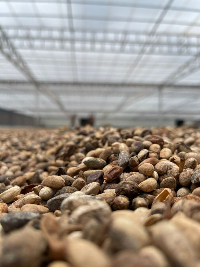
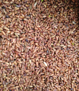
Freshly harvested neem seeds are dried under controlled conditions before processing. Proper drying helps preserve limonoid compounds critical to neem’s pesticidal properties.
Neem (Azadirachta indica) is a drought-resistant tropical tree in the Meliaceae family, native to the Indian subcontinent and parts of Southeast Asia. This multipurpose species has been used for millennia in Indian Ayurvedic medicine, much like its close relative, chinaberry, in traditional Chinese medicine, and for pest management. While neem oil and neem seeds are best known for their use in pest control, its leaves, flowers and twigs have also been used in medicine or cooking in many tropical countries. Neem-based toothpastes, soaps, face washes, skin salves and hair care products are everyday items in Cambodia, India, Indonesia, Malaysia, Thailand, Vietnam and other regions. In rural India and parts of Africa, neem twigs are used as natural toothbrushes.
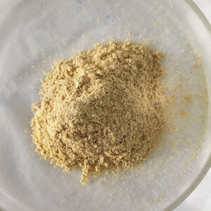
Finely ground neem seed powder is often processed into bioactive products for pest and disease management, thanks to its high azadirachtin content. (Photos K. R. Krish/Kriya Biosys Pvt. Ltd.)
The tree’s therapeutic and pesticidal properties come from the limonoid azadirachtin and other compounds found in its seeds, foliage and other parts. Limonoids are modified terpenoids present in citrus and other plants with diverse biological activity. Neem kernels contain 0.14% to 2.02% azadirachtin, while pressed oil contains 300 to 3,000 parts per million. Azadirachtin acts as an antifeedant, insect growth regulator, repellent and insecticide. It blocks the release of growth hormones ecdysone and juvenile hormone, resulting in molting disruption, and interferes with cell division, protein synthesis, reproduction and feeding. When neem oil is sprayed, the oil film itself suffocates eggs and young insects, while also preventing fungal spores from germinating, a dual barrier against pests and pathogens.
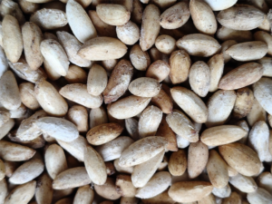
Cleaned and dehulled neem seeds are a primary source of neem oil and azadirachtin, widely used in biopesticide formulations.
After oil and azadirachtin are extracted, the remaining seed cake serves as a fertilizer or can be further processed to yield protein for amino acid and peptide extraction, as well as carbohydrates that can be used as organic manure. Gallic acid, gedunin, mahmoodin, nimbin and nimbinin from neem seed, bark or roots have antimicrobial activity. With one or more of these compounds, neem can be an important tool in plant protection.
Research-backed benefits in pest and disease control Numerous azadirachtin- and neem oil-based pesticides are sold worldwide for farms and home gardens. Their multiple modes of action, compatibility with other inputs, low mammalian toxicity and minimal risk to pollinators make them well suited for integrated pest management. There are currently 29 registered pesticides in California containing neem oil and 34 containing azadirachtin, according to the California Department of Pesticide Regulation. More than 100 neem oil-based and 37 azadirachtin-based products are registered in the United States through the U.S. Environmental Protection Agency. Some products contain combinations of these active ingredients or others, such as pyrethrins and piperonyl butoxide, which increase efficacy.
In California field studies, combining or rotating azadirachtin products with other pesticides, especially biopesticides, often delivered superior control. For example, while the entomopathogenic fungus Beauveria bassiana alone was ineffective against root aphids in organic celery, combining it with azadirachtin provided the best control among treatments evaluated. Similarly, a combination of the synthetic insect growth regulator novaluron and a pyrethroid, followed by two applications of the entomopathogenic fungus Metarhizium brunneum with azadirachtin, ranked among the top treatments for western tarnished plant bug (Lygus hesperus) in strawberry.
Variations in neem seed appearance can reflect ripeness, regional genetics or postharvest handling. These seeds will be processed into oil or used to produce neem cake.
Azadirachtin followed by abamectin or imidacloprid was as effective as abamectin followed by imidacloprid for controlling mites (Oligonychus punicae and Oligonychus perseae) in avocado in Mexico. In a Brazilian study, azadirachtin was as effective as abamectin against twospotted spider mites (Tetranychus urticae) in strawberry. Although it reduced fecundity of predatory mites (Neoseiulus californicus and Phytoseiulus macropilis), it did not significantly affect their survival. In Tunisia, neem oil extract provided up to 82 percent control of the mealy aphid complex (Hyalopterus pruni) in almonds.
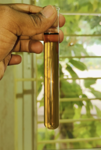
Cold-pressed neem oil, rich in azadirachtin and other active compounds, is used in registered biopesticide products and offers antifungal, antifeedant and insecticidal effects. (Photo K. R. Krish/Kriya Biosys Pvt. Ltd.)
Neem also shows promise in plant disease management. A recent Iranian study demonstrated that a high concentration of neem seed alcoholic extract resulted in 81 percent and 92 percent inhibition of anthracnose (Colletotrichum nymphaeae) and gray mold (Botrytis cinerea), respectively, in strawberry. Neem enhanced the efficacy of the microbial control agents Purpureocillium lilacinum and Trichoderma harzianum against Fusarium oxysporum f. sp. lycopersici and the root-knot nematode Meloidogyne javanica in tomato in Kenya. Similarly, soil application of crude and refined neem extracts significantly reduced root-knot nematode egg masses and egg numbers on tomato roots in England.
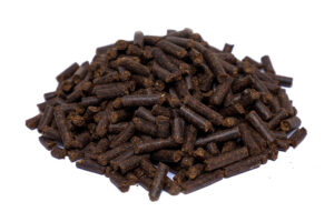
Neem seed cake, a byproduct of oil extraction, is pressed into pellets and used as an organic fertilizer with added pest-suppressive benefits. (Photo K. R. Krish/Kriya Biosys Pvt. Ltd.)
Soil fertility and yield impacts Neem also plays a role in soil fertility and crop production. A Brazilian study reported an 18 percent increase in corn yield after applying about 11 pounds per acre of neem cake as an organic fertilizer. In Nigeria, soil application of neem seed cake before planting significantly increased okra yields. However, studies in Nigeria and Egypt showed that neem seed cake, alone or combined with biochar, affected nitrogen cycling differently depending on soil type. The combination increased ammonia volatilization in neutral and alkaline soils but increased nitrification and reduced ammonia loss in acidic soils.
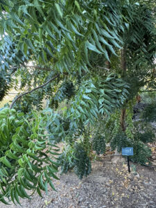
A mature neem tree (Azadirachta indica). Native to South Asia, neem thrives in warm, frost-free climates and offers a sustainable source of bioactive compounds used in pest and disease management. (Photo S. Dara)
Opportunities for U.S. growers Although limited research has been conducted in the United States, studies from around the world demonstrate neem’s potential in crop protection, soil health and nutrient management. Neem products and their active ingredients are currently imported, but domestic production could be beneficial. Arizona, California, Florida and Hawaii have warm, frost-free zones where neem trees can grow. Several Hawaiian islands already have neem planted as landscape trees, offering untapped agricultural potential. While U.S.-based production would take time to develop, currently available neem products already play a meaningful role in sustainable agriculture.
References:
Adusei, S. and S. Azupio.2022.Neem: a novel biocide for pest and disease control of plants.J. Chem. 1: 6778554. https://doi.org/10.1155/2022/6778554
Bernardi, D. et al. 2013.Effects of azadirachtin on Tetranychus urticae (Acari: Tetranychidae) and its compatibility with predatory mites (Acari: Phytoseiidae) on strawberry.Pest Manag. Sci. 69: 75-80.
Braham, M., A. Abbes, D. Benchehla.2014.Evaluation of four organically-acceptable insecticides against mealy aphids of the Hyalopterus pruni complex in almond orchard.J. Agric. Crop Res. 2: 211-217.
Cantú-Díaz et al.2016.Control of mites and thrips and its impact on the yield of avocado cv. “Hass” in Filo de Caballos, Guerrero, Mexico.Int. J. Env. Agric. Res. 2: 14-20.
Dara, S.K.2015.Root aphids and their management in organic celery. CAPCA Adviser, 18, 56–58.
Dara, S. K., D. Peck, and D. Murray.2018.Chemical and non-chemical options for managing twospotted spider mite, western tarnished plant bug and other arthropod pests in strawberries.Insects 9: 156. https://doi.org/10.3390/insects9040156
Eifediyi, E. K., K. O. Mohammed, and S. U. Remison.2015.Effects of neem (Azadirachta indica L.) seed cake on the growth and yield of okra (Abelmoschus esculentus (L.) Moench). Poljoprivreda 21: 46-52.
Jave, N., S. R. Gowen, M. Inam-ul-Haq, and S. A. Anwar.2007.Protective and curative effect of neem (Azadirachta indica) formulations on the development of root-knot nematode Meloidogyne javanica in roots of tomato plants. Crop Protec. 26: 530-534. https://doi.org/10.1016/j.cropro.2006.05.003
Mwangi, M. W., W. M. Muiru, R. D. Narla, J. W. Kimenju, and G. M. Kariuki.2018.Management of Fusarium, oxysporum f. sp. Lycopersici and root-knot nematode disease complex in tomato by use of antagonistic fungi, plant resistance and neem. Biocon. Sci. Tech. 29: 229-238. https://doi.org/10.1080/09583157.2018.1545219
Oladele, S. O., A. C. Adegaye, A. Wewe, T. M. Agbede, and A. A. Adebo.2024. Biochar and neem seed cake co-amendment effects on soil nitrogen cycling and NH3 volatilization in contrasting soils.Discover Appl. Sci. 6, 634. https://doi.org/10.1007/s42452-024-06354-7
Motallebi, P. and M. Negahban.2024.Neem (Azadirachta indica) seed extract formulation for managing anthracnose and gray mold diseases in strawberry. S. Afr. J. Bot. 169: 66-71. https://doi.org/10.1016/j.sajb.2024.04.027
Silva, J.S.L. et al. 2024.Use of neem vegetable cake (Azadirachta indica A. Juss) increases corn productivity. Braz. J. Biol. 84, e281515. https://doi.org/10.1590/1519-6984.281515
Tomé, H.V.V., J. C. Martins, A.S. Corrêa, T.V.S. Galdino, M.C. Picanço, and R.N.C. Guedes 2013.Azadirachtin avoidance by larvae and adult females of the tomato leafminer Tuta absoluta.Crop Protec. 46: 63-69.
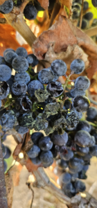
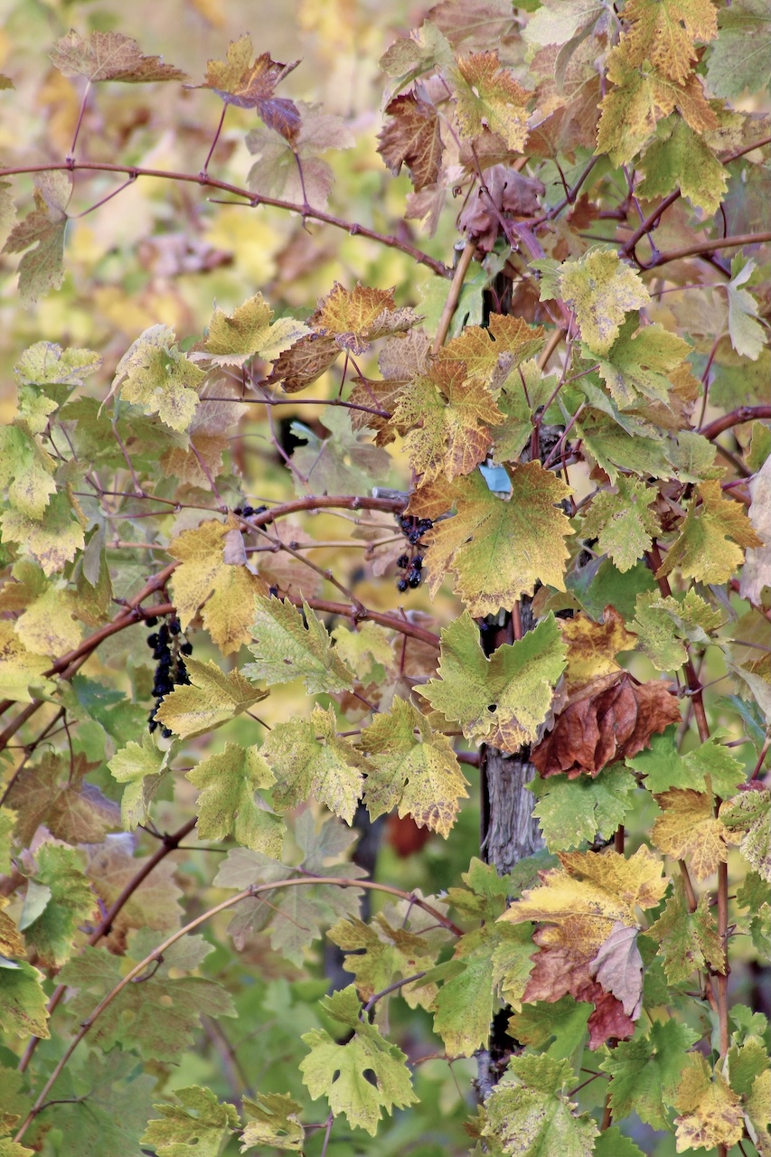
Figure 1. Clusters showing late-season rot symptoms observed on Petit Verdot in the Lodi/Clements area during the 2025 harvest. (Photo credit: C. Starr)
The 2025 growing season in California brought a cooler-than-average summer that delayed harvest across portions of the San Joaquin Valley and Napa Valley. What initially seemed like just a longer wait for sugar accumulation instead revealed an unexpected challenge: a noticeable increase in late-season fruit rots (Figure 1).
Weather data show that heat accumulated more slowly than in typical warm seasons, extending fruit development into late September and October. Several rain events occurred during this period, when berries were soft and sugar levels were still rising. In contrast, in warmer years like 2024, fruit matured earlier under dry conditions, avoiding this overlap between ripening and rainfall. The slower heat accumulation and moisture during the final weeks of 2025 created ideal conditions for fungal infection and explain the widespread appearance of unusual rots observed this year.
Growers, pest control advisers, and farm advisers reported clusters showing symptoms typical of Botrytis and Cladosporium rots (Figure 2), including in cultivars such as Cabernet Sauvignon, Zinfandel and Petit Verdot that are not usually heavily affected. These are late-ripening cultivars that require a high accumulation of growing degree days (GDD) to reach full maturity, often ripening late in the season when the likelihood of fall moisture increases. Under a cool year like 2025, the additional time needed for ripening extended fruit exposure to humid conditions, increasing the period of susceptibility.
Figure 2. Cluster infected by Cladosporium. (Photo credit: C. Starr)
Why we are seeing more Cladosporium rot Cladosporium species are common vineyard inhabitants that typically live on grape surfaces as saprophytes—fungi that grow on dead and aging plant tissue. However, under mild temperatures and high humidity, especially when harvest is delayed, they can become opportunistic pathogens. Studies from California and Chile have shown that Cladosporium species infect berries with elevated sugar levels or minor skin injuries. As berries reach full maturity, the cuticle naturally thins and loses integrity, reducing its barrier function against fungal invasion. Disease development is favored when humidity remains high and temperatures range between 68 and 77°F (20 and 25 °C).
This year’s combination of cool temperatures, extended hang time and early fall rains favored Cladosporium infection and sporulation. The fungus thrives on senescing berry tissue, producing olive-green or dark brown growth that may easily be mistaken for Botrytis. In several vineyards, both fungi were observed colonizing the same clusters (Figure 2).
‘Cool temperatures, extended hang time and early fall rains in 2025 created ideal conditions for Cladosporium rot to emerge—even in cultivars not typically affected.’
A changing climate means changing risk Seasons like 2025 are becoming more common as California’s climate grows increasingly variable. Cooler or wetter late seasons now occur in regions that traditionally experienced hot and dry ripening conditions. These shifts challenge existing fungicide programs, which are typically designed for shorter harvest periods. When harvest is delayed, the protective window of preharvest sprays may expire before fruit is picked, leaving clusters exposed during periods of high humidity or rain.
Preparing for future seasons Growers and advisers should plan for longer harvest windows as part of their disease management strategy. Some practical steps include:
• Add a late-season protective spray if harvest is delayed and rainfall or heavy dew is expected. Check preharvest intervals and rotate fungicide modes of action.
• Scout carefully before harvest to detect early signs of Cladosporium or Botrytis sporulation in shaded clusters or damaged berries.
• Maintain canopy ventilation through leaf removal and crop thinning to reduce humidity around the fruit zone.
• Use weather-based forecasting tools that track temperature, humidity and rainfall to anticipate infection risk.
Looking ahead The 2025 season highlights how quickly disease pressure can change with the weather. A proactive approach that includes careful monitoring, flexible spray programs and strong communication between growers, advisers and researchers will be essential for managing fruit rots under increasingly variable conditions.
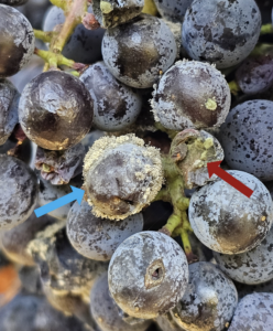
Figure 3. Mixed A of Botrytis (blue arrow) and Cladosporium (red arrow) colonizing the same cluster. (Photo credit: C. Starr)
Quick facts: Recognizing Cladosporium rot • Appearance: Olive-green to dark brown velvety growth on berry surfaces (Figure 3).
• Typical conditions: Moderate temperatures 68 to 77°F (20 to 25 °C) and high humidity, especially after rain or heavy dew.
• High-risk situations: Delayed harvest, extended hang time, tight clusters and shaded fruit zones.
• Management tip: Maintain fungicide protection when harvest is delayed and rainfall is expected.
References Briceño, E. X., and Latorre, B. A. 2008. Characterization of Cladosporium rot in grapevines, a problem of growing importance in Chile. Plant Dis. 92:1635–1642.
Crandall, S. G., Spychalla, J., Crouch, U. T., Acevedo, F. E., Naegele, R. P., and Miles, T. D. 2022. Cluster rot disease complexes, management, and future prospects. Plant Dis. 106:2013–2025.
Latorre, B. A., and Briceño, E. X. 2007. Outbreaks of Cladosporium rot associated with delayed harvest of wine grapes in Chile. Plant Dis. 91:1137.
Solairaj, D., Ngolong Ngea, G. L., Yang, Q., Liu, J., and Zhang, H. 2022. Microclimatic parameters affect Cladosporium rot development and berry quality in table grapes. Hortic. Plant J. 8:171–183.
Swett, C. L., Bourret, T., and Gubler, W. D. 2016. Characterizing the brown spot pathosystem in late-harvest table grapes in the California Central Valley. Plant Dis. 100:2204–2210.
Continuing education shapes the guidance consultants provide
every day. Early CE planning ensures they stay ahead of new
challenges and support growers with the most current information.
Dear Crop Consultant,
One thing I have learned over the years working alongside crop consultants across California is this: The best consultants never treat continuing education like a box to check. They treat it like part of their business plan.
Why CEs Matter CEs matter, not just because they are required to keep your license current, but because this industry never sits still. Products change. Research advances. Regulations evolve. The consultants who stay ahead are the ones who make education intentional and easy, instead of something they scramble to finish late in the year.
Every season, we hear the same comments: “I still need credits.” “Everything is booked.” “I have been too busy to think about it.” And honestly, that is understandable. You are in the field, meeting with growers, managing real problems and making decisions that matter. Education often slips down the list until it suddenly becomes urgent.
That is exactly why planning early is so important.
As the publisher of Progressive Crop Consultant magazine and host of the Crop Consultant Conference, I want to personally encourage you to make your CE plan now and make it simple. This conference was built specifically for crop consultants who want practical, relevant education without the hassle.
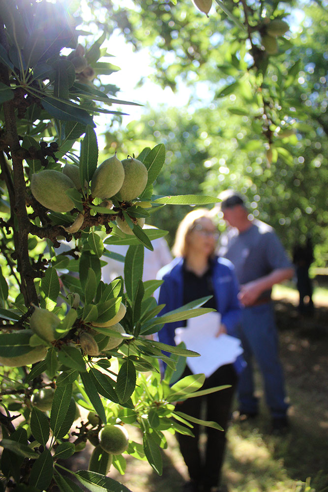
Strong field decisions start with up-to-date knowledge. Planning early for CE opportunities helps consultants bring the latest research and best practices back to the orchard. (Photos K. Platts)
One Event, Real Benefits For $350, you can attend the Crop Consultant Conference and take care of your education in one place, at one event, with content that actually applies to what you see in the field. One registration. One trip. No chasing credits. No juggling multiple meetings.
That price is intentional. We want education to be accessible and straightforward. We want consultants to feel good about investing in themselves without overthinking it. When you compare that cost to fuel, travel time or attending multiple smaller events throughout the year, this becomes one of the easiest professional decisions you can make.
More importantly, it saves you time.
Instead of piecing together credits from different events, you show up knowing your education is handled. You sit in sessions focused on real-world agronomy, current research, regulatory updates and issues that matter to California agriculture. You hear from people who understand your role and respect your time.
That peace of mind matters during a busy season.
Education also does more than keep you compliant. It strengthens your confidence. It sharpens your recommendations. It gives you current talking points when you are sitting across the table from a grower making important decisions. Staying educated directly impacts how you are perceived in the field.
Growers notice when their consultant is informed. They notice when recommendations are grounded in solid research and current insight. They notice when you can clearly explain changes, risks and opportunities. Education reinforces your credibility, and credibility builds long-term trust.
The Crop Consultant Conference is also about being in the room with peers who do what you do every day. There is real value in hearing what other consultants are seeing, what challenges they are facing and how they are adapting. Those conversations often end up being just as valuable as the sessions themselves.
At JCS Marketing, our goal has always been to make education useful and efficient. No filler sessions. No wasted time. Just solid content delivered by people who understand the industry and respect the realities of your schedule.
Waiting until later in the year almost always makes things harder. Registration fills up. Calendars tighten. Costs increase. Planning early gives you control. You lock it in, move on and focus on your work knowing your CE requirements are covered.
For $350, you are buying simplicity. You are buying convenience. You are buying confidence that your education is handled without stress. That is a small investment compared to the value of staying current and professional in a fast-moving industry.
Plan Now, Avoid the Scramble My advice is simple: Do not make CEs harder than they need to be. Choose an option that respects your time, fits your budget and delivers real value. Make the plan now so you are not scrambling later.
We would love to have you join us at the Crop Consultant Conference this September. Secure your spot early, get your education lined up and give yourself one less thing to worry about as the season ramps up.
Fungicides are usually applied during bloom to protect blossoms from becoming infected. Fungicides should be selected carefully to avoid resistance and to control the pathogens present. (Photo courtesy UCCE)
Almond growers have a narrow window from pink bud to petal fall to prevent outbreaks of bacterial and fungal diseases. UC IPM guidelines note that monitoring environmental factors during the critical period and knowing the disease history of specific orchards are important components to understanding the orchard needs and to prevent yield losses due to disease.
Depending on the level of disease inoculum present in the orchard, rainfall and warm temperatures can significantly increase the likelihood of a severe and widespread infection that will affect production. Dry weather during and right after bloom reduces the risk of serious infection. Spores are airborne or rain-splashed, and infection is favored when temperatures are in the mid-70s during bloom. Humid conditions can contribute to the chance of a disease outbreak. Preventive steps in the face of environmental conditions conducive to bloom disease outbreaks can be the difference between good almond production and severe yield loss.
The main fungal diseases in almonds at bloom are brown rot blossom blight, green fruit rot or jacket rot, and shothole. Less prevalent are scab, rust, leaf blight and anthracnose. According to UCCE San Joaquin County farm advisor Brent Holtz, the pathogens that cause these diseases are usually present in the orchard. The levels of inoculum possible this year depend on the past year’s disease levels. Environmental conditions, temperatures and moisture trigger disease development in the presence of the pathogen.
A successful prevention program is based on informed choice of fungicide, good timing of application and optimum coverage. Combinations of fungicides are commonly used to cover the spectrum of pathogens.
Brown Rot
Warm temperatures and enough dew formation can initiate a brown rot outbreak. A dry winter is no guarantee that brown rot won’t occur in the orchard. Decisions to make preventive spray applications should be based on history of disease in the orchard and weather predictions. In young orchards without any significant disease history, decisions for spray applications should be considered to prevent buildup of inoculum, particularly if older orchards are nearby.
There are specific conditions that favor bloom disease development. For blossom infection to occur at 50 degrees Fahrenheit, 18 hours of leaf wetness is needed. At a higher temperature of 68 degrees, only eight hours of leaf wetness is needed. High humidity affects disease symptom development. Spore masses can form on flower parts. The stamens and pistils are the most susceptible parts of the flower.
Timing fungicide applications is critical to prevention. According to UC, brown rot infection timing is from pink bud through petal fall. Full blooms are most susceptible. Two fungicide applications are normal for brown rot prevention. The first is done at 5 to 20 bloom with a systemic. The second, a rotation, is at 80% bloom or two weeks after the first. If wet weather persists, a third could be warranted. In dry conditions, a single application at 20 to 40% bloom is recommended.
Green Fruit Rot or Jacket Rot
Favorable conditions for infection are cool, wet weather and nut clusters that trap senescing flower parts. The pathogen moves into the jackets, damaging the nut embryo. Fungicide application timing is full bloom and when bloom is extended.
Shothole
This is a later bloom disease that infects leaves, fruits and green wood. Leaf infections result in a lesion with a yellow halo. The lesion later leaves a hole in the leaf. Severe infection can kill the developing nut or cause kernel deformities. The condition occurs with moisture and temperatures above 36 degrees Fahrenheit. It is common when significant rain occurs after leaf-out. The UC guidelines note the life cycle and fungicides for control.
Anthracnose
This disease is less common. It is triggered by warm, wet spring weather. Prevention should begin from pink tip forward to protect blossoms.
Bacterial Disease
Bacterial blast is low risk in dry years, but can cause significant damage in wet and freezing temperatures. Symptoms are shriveled blossoms. Buds can die, and dieback can occur on larger branches with severe infections.
A Section 18 request was granted for use of kasugamycin to prevent spread of the disease.
Honeybee protection is a concern with use of fungicides during bloom when bees are present. Applications should be made when bees are not actively foraging.
The threecornered alfalfa hopper (Spissistilus festinus) is a known vector of Grapevine red blotch virus, transmitting the pathogen as it feeds on vine tissues (Photo J. Kelly Clark, courtesy UC Statewide IPM Program.)
A diagnostic tool to determine whether grapevines are infected with the viral Grapevine red blotch virus (GRBV) has been developed by University of California researchers. Dr. Monica Cooper, UCCE viticulture advisor, noted that early detection of this incurable grapevine disease allows for removal of infected vines and reduces the level of inoculum in the vineyard.
Grapevine red blotch disease was first detected at the UC Davis Oakville research station in 2007 but was not formally identified until 2012. Cooper, speaking in a UC Experts Talk webinar, said the disease may have evolved in California from a latent virus found in native grapes. The virus infects plants in the Vitaceae family, including cultivated grape varieties. The disease has been found in many wine grape varieties and is believed to infect table grapes, raisin grapes and rootstock.
Vines infected with GRBV show symptoms similar to vine leafroll disease, with leaves turning red in early fall, primarily at the base of shoots. Unlike leafroll, red blotchinfected vines have red or pink veins in the leaves, red blotches on the leaves and no leafroll. Visual mapping of infected vines can be tricky, Cooper said, because symptoms can vary by cultivar, location or season.
Disease impacts fruit quality
Infected vines have an economic impact on vineyards, producing fruit that is often unsuitable for market. The disease reduces sugar accumulation, increases malic acid and less consistently increases pH and titratable acidity. Cluster weight can be reduced.
Cooper noted there are two ways the disease spreads in vineyards: through grafts using infected plant material or via the threecornered alfalfa hopper (Spissistilus festinus). Currently the only treatment is vine removal.
In the webinar, Cooper discussed the loopmediated isothermal amplification (LAMP) tool. Growers, vineyard managers or crop consultants can use this inhome assay to detect the presence of GRBV in vines without sending samples to a diagnostic lab. The LAMP tool detects and amplifies viral DNA from GRBVinfected vines. The amplification causes a color change used to interpret results.
Symptoms of Grapevine red blotch virus can include irregular red blotches on leaves and delayed ripening, which may be mistaken for other vine diseases (E. Kilmartin, UC Agricultural and Natural Resources.)
Sampling steps
Plant material can be collected from petioles, canes or vine trunks. Petioles can be sampled for the LAMP assay from veraison to just before presenescence. Once leaves begin to yellow, they are not suitable sample material. Canes can be sampled from presenescence to pruning. Cooper said canederived samples can be stored in a freezer for a short time, and petiole samples can be refrigerated for up to a week before use. Trunk material can be sampled at any time during the year.
Location on the plant where the sample is taken matters. Cooper noted that GRBV is unevenly distributed within grapevines. Studies have shown that basal tissue or older tissue is more reliable and less likely to result in false negatives. For example, samples should be taken from both sides of a bilateral cordon. She recommended collecting samples from multiple locations on a vine for best representation of disease status.
With trunk or cane material, Cooper said to peel back the outer bark and use a pipette to collect a sample from the vascular tissue. The sample placed in a test tube serves as the sample template. The next step is to mix the reagents and dispense them into PCR tubes. The reagents include primers, distilled water and Master Mix, which is used to elicit the color change. The final step is to add the samples to each tube and close them tightly. The tubes are then placed in a heat block for about 35 minutes. During that time the amplification takes place, resulting in the color change.
Once removed from the heat block, any tube with a yellow color indicates the sample is positive for GRBV. All negative controls remain pink.
This method of testing grapevine tissue samples for the presence of GRBV requires attention to detail, Cooper said, because there is a high risk of contamination. Cleaning workspaces and all equipment thoroughly with a bleach solution can help prevent contamination. Cooper noted there is a learning curve with this testing method, but with careful technique it can be mastered.
Brandon, Manitoba (December 2, 2025) – Bushel Plus Ltd., a global leader in harvest optimization solutions, announces a strategic partnership with John Deere, making the Bushel Plus SmartPan™ System available to U.S. and Canadian farmers through John Deere’s North American dealer network.
This collaboration brings together Bushel Plus’s proven drop-pan measurement system and John Deere’s advanced Harvest Settings Automation technology – giving farmers precise data to minimize harvest loss, optimize combine performance, and increase profitability.
“John Deere and Bushel Plus share a commitment to innovation and farmer success,” said Ryan Krogh, Global Combine and FEE Business Manager at John Deere. “Our decision to partner was driven by aligned values – both companies prioritize solutions that empower growers to maximize efficiency and profitability. This partnership is an important step for us to give our customers access and training to use the SmartPan System in combination with the Harvest Settings Automation technology, giving producers the tools they need to reduce harvest losses and make data‑driven decisions with confidence.”
SmartPan System: The Ground-Truth Layer that Enhances Automation John Deere’s Harvest Settings Automation automatically adjusts key combine parameters – including rotor speed, fan speed, concave clearance, and sieve and chaffer settings – in real time to maintain operator-defined limits for grain loss, broken grain, and foreign material.
The Bushel Plus SmartPan System works in tandem with John Deere’s Harvest Settings Automation to optimize efficiency during harvesting. The SmartPan System provides the ground truth data for the loss target number calibration within the Harvest Settings Automation screen. By delivering reliable measurements, the SmartPan System empowers operators to fine-tune harvest settings, significantly improving overall efficiency and reducing grain loss.
By physically collecting and calculating true bushels-per-acre losses, the SmartPan System provides farmers with the real-world verification to calibrate and validate their automated settings. This ensures that the combine’s loss limits and adjustment strategies align with actual field results.
Farmers can drop the pan at any point during harvest, compare SmartPan results to their John Deere G5Plus display, and adjust machine settings accordingly. Harvest Settings Automation automatically adjusts settings across changing crop and field conditions to maximize productivity while keeping losses below the operator-defined loss limit.
Broad Access Through Deere Dealers Under this new agreement, John Deere dealers across the U.S. and Canada will be authorized to sell and support the SmartPan System, giving farmers streamlined access through the same trusted dealer network they rely on for combine sales, service, and technology integration.
“We are excited to partner with John Deere, marking a major milestone in our growth and global reach,” says Marcel Kringe, founder and CEO of Bushel Plus. “John Deere’s commitment to innovation, as the world’s largest manufacturer of agricultural equipment, aligns perfectly with our mission to deliver market-leading harvest optimization solutions and technology. This milestone showcases our team’s global efforts and the trust farmers place in our technology. The positive feedback we receive—showing that our solutions deliver real value and profitability—is truly humbling. With OEM endorsement, the phrase ‘you can’t manage what you don’t measure’ reaches a whole new level.”
John Deere’s dealer-led distribution ensures broad access, timely support, and seamless integration of the Bushel Plus SmartPan System with its existing combine technology. In 2026, Bushel Plus and John Deere will collaborate on joint training sessions, in-field demos, and educational events to help operators understand how the SmartPan System works alongside automation to improve harvest precision.
Converging Data, Better Decisions According to Kringe, the SmartPan System provides farmers with immediate, actionable intelligence that directly strengthens harvest precision, equipment and labor efficiency, and crop management decisions.
“Seed-to-harvest precision is only as good as the data behind it,” says Kringe. “By working hand-in-hand with John Deere, we’re delivering a streamlined flow of data between field measurements and machine analytics, enabling farmers to refine combine calibration and automation for more efficient harvesting, reduced grain loss, and ultimately higher profitability.”
The Bushel Plus SmartPan System supports a wide range of crops, including corn, soybeans, wheat, canola, barley, rice, and milo, and is available in 20-inch, 40-inch, and 60-inch pan sizes to accommodate various John Deere combine models, stubble conditions, and header widths.
For more information, farmers can contact their local John Deere dealer or visit bushelplus.com.
###
SmartPan™ System is a trademark of Bushel Plus Ltd. G5Plus and John Deere are trademarks of Deere & Company.
About Bushel Plus Bushel Plus Ltd., a global leader in harvest optimization technology, specializes in solutions that help growers reduce grain loss and maximize yield potential at harvest. Trusted in more than 40 countries, Bushel Plus partners with dealers, agronomists, and equipment manufacturers to improve harvest outcomes for farmers. Guided by the belief that ‘you can only harvest once,’ the company equips farmers with field-proven tools that turn invisible losses into visible profit. To learn more, visit us at bushelplus.com.


 Invading California")

