Fungicides are usually applied during bloom to protect blossoms from becoming infected. Fungicides should be selected carefully to avoid resistance and to control the pathogens present. (Photo courtesy UCCE)
Almond growers have a narrow window from pink bud to petal fall to prevent outbreaks of bacterial and fungal diseases. UC IPM guidelines note that monitoring environmental factors during the critical period and knowing the disease history of specific orchards are important components to understanding the orchard needs and to prevent yield losses due to disease.
Depending on the level of disease inoculum present in the orchard, rainfall and warm temperatures can significantly increase the likelihood of a severe and widespread infection that will affect production. Dry weather during and right after bloom reduces the risk of serious infection. Spores are airborne or rain-splashed, and infection is favored when temperatures are in the mid-70s during bloom. Humid conditions can contribute to the chance of a disease outbreak. Preventive steps in the face of environmental conditions conducive to bloom disease outbreaks can be the difference between good almond production and severe yield loss.
The main fungal diseases in almonds at bloom are brown rot blossom blight, green fruit rot or jacket rot, and shothole. Less prevalent are scab, rust, leaf blight and anthracnose. According to UCCE San Joaquin County farm advisor Brent Holtz, the pathogens that cause these diseases are usually present in the orchard. The levels of inoculum possible this year depend on the past year’s disease levels. Environmental conditions, temperatures and moisture trigger disease development in the presence of the pathogen.
A successful prevention program is based on informed choice of fungicide, good timing of application and optimum coverage. Combinations of fungicides are commonly used to cover the spectrum of pathogens.
Brown Rot
Warm temperatures and enough dew formation can initiate a brown rot outbreak. A dry winter is no guarantee that brown rot won’t occur in the orchard. Decisions to make preventive spray applications should be based on history of disease in the orchard and weather predictions. In young orchards without any significant disease history, decisions for spray applications should be considered to prevent buildup of inoculum, particularly if older orchards are nearby.
There are specific conditions that favor bloom disease development. For blossom infection to occur at 50 degrees Fahrenheit, 18 hours of leaf wetness is needed. At a higher temperature of 68 degrees, only eight hours of leaf wetness is needed. High humidity affects disease symptom development. Spore masses can form on flower parts. The stamens and pistils are the most susceptible parts of the flower.
Timing fungicide applications is critical to prevention. According to UC, brown rot infection timing is from pink bud through petal fall. Full blooms are most susceptible. Two fungicide applications are normal for brown rot prevention. The first is done at 5 to 20 bloom with a systemic. The second, a rotation, is at 80% bloom or two weeks after the first. If wet weather persists, a third could be warranted. In dry conditions, a single application at 20 to 40% bloom is recommended.
Green Fruit Rot or Jacket Rot
Favorable conditions for infection are cool, wet weather and nut clusters that trap senescing flower parts. The pathogen moves into the jackets, damaging the nut embryo. Fungicide application timing is full bloom and when bloom is extended.
Shothole
This is a later bloom disease that infects leaves, fruits and green wood. Leaf infections result in a lesion with a yellow halo. The lesion later leaves a hole in the leaf. Severe infection can kill the developing nut or cause kernel deformities. The condition occurs with moisture and temperatures above 36 degrees Fahrenheit. It is common when significant rain occurs after leaf-out. The UC guidelines note the life cycle and fungicides for control.
Anthracnose
This disease is less common. It is triggered by warm, wet spring weather. Prevention should begin from pink tip forward to protect blossoms.
Bacterial Disease
Bacterial blast is low risk in dry years, but can cause significant damage in wet and freezing temperatures. Symptoms are shriveled blossoms. Buds can die, and dieback can occur on larger branches with severe infections.
A Section 18 request was granted for use of kasugamycin to prevent spread of the disease.
Honeybee protection is a concern with use of fungicides during bloom when bees are present. Applications should be made when bees are not actively foraging.
The threecornered alfalfa hopper (Spissistilus festinus) is a known vector of Grapevine red blotch virus, transmitting the pathogen as it feeds on vine tissues (Photo J. Kelly Clark, courtesy UC Statewide IPM Program.)
A diagnostic tool to determine whether grapevines are infected with the viral Grapevine red blotch virus (GRBV) has been developed by University of California researchers. Dr. Monica Cooper, UCCE viticulture advisor, noted that early detection of this incurable grapevine disease allows for removal of infected vines and reduces the level of inoculum in the vineyard.
Grapevine red blotch disease was first detected at the UC Davis Oakville research station in 2007 but was not formally identified until 2012. Cooper, speaking in a UC Experts Talk webinar, said the disease may have evolved in California from a latent virus found in native grapes. The virus infects plants in the Vitaceae family, including cultivated grape varieties. The disease has been found in many wine grape varieties and is believed to infect table grapes, raisin grapes and rootstock.
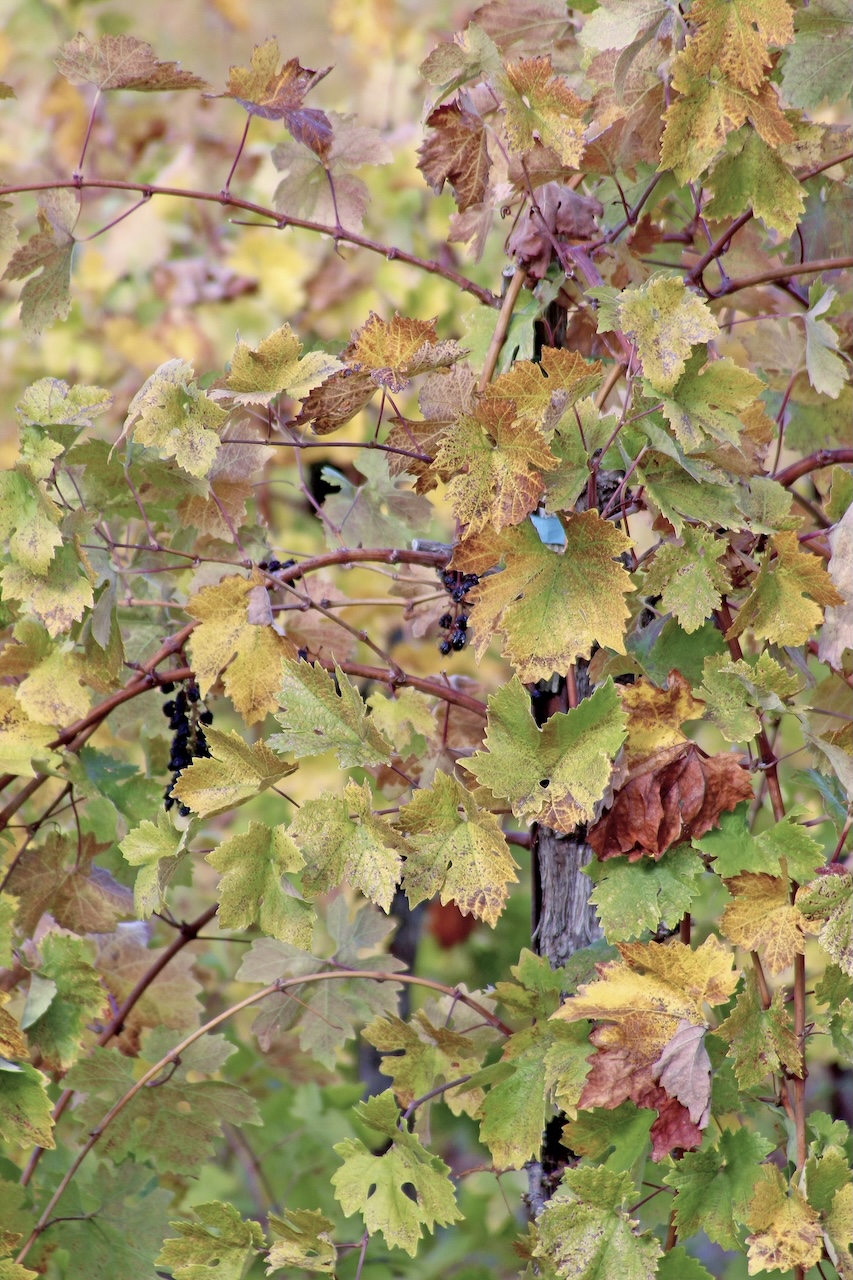
Vines infected with GRBV show symptoms similar to vine leafroll disease, with leaves turning red in early fall, primarily at the base of shoots. Unlike leafroll, red blotchinfected vines have red or pink veins in the leaves, red blotches on the leaves and no leafroll. Visual mapping of infected vines can be tricky, Cooper said, because symptoms can vary by cultivar, location or season.
Disease impacts fruit quality
Infected vines have an economic impact on vineyards, producing fruit that is often unsuitable for market. The disease reduces sugar accumulation, increases malic acid and less consistently increases pH and titratable acidity. Cluster weight can be reduced.
Cooper noted there are two ways the disease spreads in vineyards: through grafts using infected plant material or via the threecornered alfalfa hopper (Spissistilus festinus). Currently the only treatment is vine removal.
In the webinar, Cooper discussed the loopmediated isothermal amplification (LAMP) tool. Growers, vineyard managers or crop consultants can use this inhome assay to detect the presence of GRBV in vines without sending samples to a diagnostic lab. The LAMP tool detects and amplifies viral DNA from GRBVinfected vines. The amplification causes a color change used to interpret results.
Symptoms of Grapevine red blotch virus can include irregular red blotches on leaves and delayed ripening, which may be mistaken for other vine diseases (E. Kilmartin, UC Agricultural and Natural Resources.)
Sampling steps
Plant material can be collected from petioles, canes or vine trunks. Petioles can be sampled for the LAMP assay from veraison to just before presenescence. Once leaves begin to yellow, they are not suitable sample material. Canes can be sampled from presenescence to pruning. Cooper said canederived samples can be stored in a freezer for a short time, and petiole samples can be refrigerated for up to a week before use. Trunk material can be sampled at any time during the year.
Location on the plant where the sample is taken matters. Cooper noted that GRBV is unevenly distributed within grapevines. Studies have shown that basal tissue or older tissue is more reliable and less likely to result in false negatives. For example, samples should be taken from both sides of a bilateral cordon. She recommended collecting samples from multiple locations on a vine for best representation of disease status.
With trunk or cane material, Cooper said to peel back the outer bark and use a pipette to collect a sample from the vascular tissue. The sample placed in a test tube serves as the sample template. The next step is to mix the reagents and dispense them into PCR tubes. The reagents include primers, distilled water and Master Mix, which is used to elicit the color change. The final step is to add the samples to each tube and close them tightly. The tubes are then placed in a heat block for about 35 minutes. During that time the amplification takes place, resulting in the color change.
Once removed from the heat block, any tube with a yellow color indicates the sample is positive for GRBV. All negative controls remain pink.
This method of testing grapevine tissue samples for the presence of GRBV requires attention to detail, Cooper said, because there is a high risk of contamination. Cleaning workspaces and all equipment thoroughly with a bleach solution can help prevent contamination. Cooper noted there is a learning curve with this testing method, but with careful technique it can be mastered.
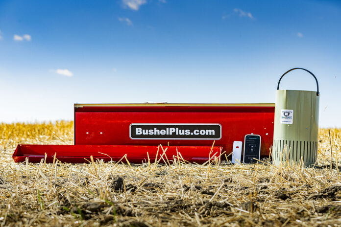
Brandon, Manitoba (December 2, 2025) – Bushel Plus Ltd., a global leader in harvest optimization solutions, announces a strategic partnership with John Deere, making the Bushel Plus SmartPan™ System available to U.S. and Canadian farmers through John Deere’s North American dealer network.
This collaboration brings together Bushel Plus’s proven drop-pan measurement system and John Deere’s advanced Harvest Settings Automation technology – giving farmers precise data to minimize harvest loss, optimize combine performance, and increase profitability.
“John Deere and Bushel Plus share a commitment to innovation and farmer success,” said Ryan Krogh, Global Combine and FEE Business Manager at John Deere. “Our decision to partner was driven by aligned values – both companies prioritize solutions that empower growers to maximize efficiency and profitability. This partnership is an important step for us to give our customers access and training to use the SmartPan System in combination with the Harvest Settings Automation technology, giving producers the tools they need to reduce harvest losses and make data‑driven decisions with confidence.”
SmartPan System: The Ground-Truth Layer that Enhances Automation John Deere’s Harvest Settings Automation automatically adjusts key combine parameters – including rotor speed, fan speed, concave clearance, and sieve and chaffer settings – in real time to maintain operator-defined limits for grain loss, broken grain, and foreign material.
The Bushel Plus SmartPan System works in tandem with John Deere’s Harvest Settings Automation to optimize efficiency during harvesting. The SmartPan System provides the ground truth data for the loss target number calibration within the Harvest Settings Automation screen. By delivering reliable measurements, the SmartPan System empowers operators to fine-tune harvest settings, significantly improving overall efficiency and reducing grain loss.
By physically collecting and calculating true bushels-per-acre losses, the SmartPan System provides farmers with the real-world verification to calibrate and validate their automated settings. This ensures that the combine’s loss limits and adjustment strategies align with actual field results.
Farmers can drop the pan at any point during harvest, compare SmartPan results to their John Deere G5Plus display, and adjust machine settings accordingly. Harvest Settings Automation automatically adjusts settings across changing crop and field conditions to maximize productivity while keeping losses below the operator-defined loss limit.
Broad Access Through Deere Dealers Under this new agreement, John Deere dealers across the U.S. and Canada will be authorized to sell and support the SmartPan System, giving farmers streamlined access through the same trusted dealer network they rely on for combine sales, service, and technology integration.
“We are excited to partner with John Deere, marking a major milestone in our growth and global reach,” says Marcel Kringe, founder and CEO of Bushel Plus. “John Deere’s commitment to innovation, as the world’s largest manufacturer of agricultural equipment, aligns perfectly with our mission to deliver market-leading harvest optimization solutions and technology. This milestone showcases our team’s global efforts and the trust farmers place in our technology. The positive feedback we receive—showing that our solutions deliver real value and profitability—is truly humbling. With OEM endorsement, the phrase ‘you can’t manage what you don’t measure’ reaches a whole new level.”
John Deere’s dealer-led distribution ensures broad access, timely support, and seamless integration of the Bushel Plus SmartPan System with its existing combine technology. In 2026, Bushel Plus and John Deere will collaborate on joint training sessions, in-field demos, and educational events to help operators understand how the SmartPan System works alongside automation to improve harvest precision.
Converging Data, Better Decisions According to Kringe, the SmartPan System provides farmers with immediate, actionable intelligence that directly strengthens harvest precision, equipment and labor efficiency, and crop management decisions.
“Seed-to-harvest precision is only as good as the data behind it,” says Kringe. “By working hand-in-hand with John Deere, we’re delivering a streamlined flow of data between field measurements and machine analytics, enabling farmers to refine combine calibration and automation for more efficient harvesting, reduced grain loss, and ultimately higher profitability.”
The Bushel Plus SmartPan System supports a wide range of crops, including corn, soybeans, wheat, canola, barley, rice, and milo, and is available in 20-inch, 40-inch, and 60-inch pan sizes to accommodate various John Deere combine models, stubble conditions, and header widths.
For more information, farmers can contact their local John Deere dealer or visit bushelplus.com.
###
SmartPan™ System is a trademark of Bushel Plus Ltd. G5Plus and John Deere are trademarks of Deere & Company.
About Bushel Plus Bushel Plus Ltd., a global leader in harvest optimization technology, specializes in solutions that help growers reduce grain loss and maximize yield potential at harvest. Trusted in more than 40 countries, Bushel Plus partners with dealers, agronomists, and equipment manufacturers to improve harvest outcomes for farmers. Guided by the belief that ‘you can only harvest once,’ the company equips farmers with field-proven tools that turn invisible losses into visible profit. To learn more, visit us at bushelplus.com.
Seasonal effort supports ongoing efforts to strengthen walnut relevance year round
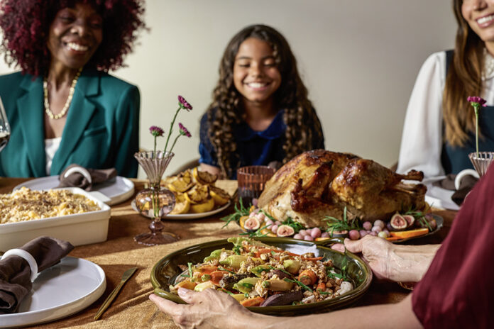
FOLSOM, Calif., Nov. 25, 2025 – The California Walnut Board and Commission is launching its “Be Merry. Feel Good.” holiday campaign in the US market to reach consumers during the year’s peak season for walnut purchases, when consumers seek ingredients for seasonal recipes and entertaining.
The campaign builds on the industry’s “California Walnuts. Feel Good.” consumer effort, which aims to modernize the image of California walnuts and reposition them as a must-have ingredient. Complete with a fresh, energetic visual identity, the industry-wide effort is expanding the target audience to include millennial and Gen Z consumers while enhancing engagement with existing consumers who already know and love California walnuts.
“The holidays are a critical time for the nut category, and this program helps ensure walnuts remain visible and top of mind when consumers are making purchase decisions,” said Christine Lott, director of integrated communications for the California Walnut Board and Commission. “During the holidays, gatherings of friends and family over a meal are one of the ways people celebrate and find joy. California walnuts are a great fit for the occasion, providing a feel-good ingredient that can elevate your holiday dishes. Our “Be Merry” campaign brings this to life, supported with retail promotions and in-store activity, while continuing to spark excitement around walnuts for the long haul.”
Retail support includes seasonal displays, tagged ads and in-store promotions. Beyond the retail environment, the campaign includes partnerships with social media influencers in cooking, wellness, lifestyle and entertaining. Paid advertising extends reach across connected TV, YouTube, podcasts and social channels and consumer publications. The Board and Commission are also reaching consumers in real life through experiential events that allow consumers to taste and learn about walnuts’ flavor and nutritional benefits.
California walnut growers and handlers can get the latest on the marketing efforts of the Board and Commission by signing up for the industry newsletter at walnuts.org/industry-subscribe/.
About the California Walnut Board and Commission The California Walnut Board (CWB) and California Walnut Commission (CWC) represent more than 3,700 California walnut growers and approximately 70 handlers, grown in multi-generational farmers’ family orchards. California walnuts, known for their excellent nutritional value and quality, are shipped around the world all year long, with more than 99% of the walnuts grown in the United States being from California.
The CWB, established in 1948, promotes usage of walnuts in the United States through publicity and educational programs. The CWB also provides funding for walnut production, food safety and post-harvest research. The CWC, established in 1987, is involved in health research with consuming walnuts as well as domestic and export market development activities.
To explore recipes and learn more about California walnut growers, industry information and health research, visit walnuts.org.
The California Plant and Soil Conference will be held on February 3-4 at the Visalia Convention Center 303 E. Acequia, Visalia, CA 93291
The conference is organized by the California Chapter of the American Society of Agronomy (CA ASA). Registration is now open through the conference website (https://na.eventscloud.com/plantandsoilconference).
The annual conference provides an opportunity for students, professionals, and other attendees to increase their knowledge of current topics of agronomic importance in California. Many Certified Crop Advisers and Pest Control Advisers attend the conference to earn continuing education units that are important to their professional standing.
This year’s conference will convene sessions covering the following topics:
The State of California Agriculture in 2026 and Beyond
Precision Ag
Integrated Pest Management
Robotics
Nutrient Management
Technology for Irrigation Management
Tools for Soil Health and Regenerative Ag
Circular Economies
Frontiers in Genetic Engineering
Crop Diversification
Groundwater Quantity and Quality for Agriculture
In addition to presentations on these topics, there will be an award ceremony to honor individuals who served the profession through their careers, a student poster competition, non-competitive professional posters, a student mentoring breakfast, and the CA ASA business meeting. Sponsorship opportunities are available to support student participation; please see the conference website for more information (https://na.eventscloud.com/website/58588/sponsors/). Early bird registration is available through January 10th.
The conference is planned and presented by a team of volunteer professional agronomists from research institutions, cooperative extension, public agencies, and private companies. If you are interested in serving on the board, or have questions about the conference, please contact a current board member (https://na.eventscloud.com/website/58588/leadership/).
The CA ASA organization was founded in April 1971 by a group of California agronomists who recognized the value in creating a forum to focus on California agriculture. The purpose of the annual meeting is to promote research, disseminate scientific information, foster high standards of educational and ethical conduct in the profession, and facilitate robust cooperation among organizations with similar missions.
Carpophilus beetle on a harvest-ready almond. Researchers are using pheromone traps and field surveys to study beetle activity and inform management strategies (photo by Mel Machado, Blue Diamond Growers.)
Carpophilus beetle, specifically Carpophilus truncatus, is a newer invasive pest making its presence known in almond and pistachio orchards across the San Joaquin Valley. First confirmed in 2023, Carpophilus beetle has been found in multiple orchards and is causing growing concern among researchers and consultants.
Almonds appear to be the beetle’s favorite host, though pistachios are likely a close second. “Very rarely we’re finding [them] in walnut orchards,” said Jhalendra Rijal, UCCE IPM advisor, “but pistachio and almonds are definitely susceptible.”
Building California Data
Because Carpophilus beetle is a relatively new pest to California, researchers have relied on studies from Australia (which has dealt with the pest for over a decade) to help form a starting point for local research.
Since detection, Rijal, who is based in the San Joaquin Valley, and other researchers have launched a wide-ranging study into the beetle’s biology and behavior in California conditions.
“We’re doing a lot of different research, figuring out their biology, field ecology, seasonal ecology, how we can potentially develop monitoring tools,” he said. “And if there are any other tools like insecticides and other things that would work.”
Pheromone Trap Shows Promise for Future Control
Among the more promising developments is a pheromone-based monitoring tool designed specifically for Carpophilus truncatus.
Traps using this pheromone, combined with a co-attractant, are already pulling in significant beetle counts in test orchards.
“It’s working really well. But so far … we’re using this as a monitoring tool,” Rijal said. “Potentially in the future, there might be the opportunity to work as a trap and kill or bait type of thing. We’re not there yet, but at least we have discovered this pheromone, and now we are testing its effectiveness in California orchards. Thanks to the researchers from Australia who discovered the pheromone, we are working collaboratively to test the lure in California and Australia.”
Rijal noted while the pheromone is not commercially available yet, hopefully it will be available in the next one to two years.
Winter Sanitation Remains the Foundation
In the absence of effective chemical controls, cultural practices, especially winter sanitation, remain the most important control tools available.
“Based on my experience in the last two, three seasons in the Northern San Joaquin Valley, a lot of orchards have Carpophilus beetle damage,” Rijal said. “I also basically see that if you have really good winter sanitation practices, then you will reduce the pressure in the orchard.”
Rijal explained that the beetles overwinter as adults in mummy nuts, particularly those on the ground.
“They actually build their population on the ground until they’re ready to infest on the hull split nut,” he said. “Because of that, you have mummy nuts as really the source where they can breed and build their population and cause higher damage.”
Rijal emphasized that sanitation is the most fundamental method of any Carpophilus management plan.
“I can’t imagine controlling Carpophilus beetle without doing winter sanitation,” he said. “And that’s the basis, that’s the first step.”
Rijal noted that sanitation efforts also suppress other pests, including navel orangeworm (NOW).
“You are not only controlling Carpophilus beetle, but also navel orangeworm with one stone, two birds,” he said. “So really, that should be the basic standard practice that at least the almond and pistachio nut crop growers should adopt.”
Identification Resources Available
With increasing reports of damage, proper pest identification is critical. Rijal and his team have developed a pictorial guide comparing Carpophilus beetle to navel orangeworm and ants at various life stages.
“[Growers and consultants] can find those, if they Google it, the guidelines for Carpophilus beetle in California orchards,” he said. “It’s also housed in one of my websites, ipmcorner.com. It’s also replicated or put out by Sacramento Valley Orchard Source.”
Rijal encouraged consultants to share the pest identification resources and to direct questions to local farm advisors.
He stressed that managing Carpophilus beetle requires collaboration across the industry.
“It’s a group effort because it’s become a bigger issue that we cannot tackle in one way,” Rijal said. “There is a lot of variability in terms of the environment. And the Carpophilus beetle seems to be highly influenced by that.”
With environmental conditions like rainfall, which favors the Carpophilus beetle population, playing a role in population dynamics, region-specific approaches may be necessary. Soggy or moldy mummy nuts, which are often found on the orchard floor due to moist and humid conditions, significantly help Carpophilus beetle survival until the fresh hull split nuts are ready.
“That’s why we kind of team up and are doing this work up and down the valley,” Rijal said.
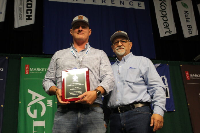
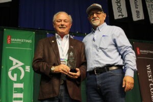
This year’s CCA of the Year winner was Eric Pooler, vice president of viticulture, winery relations and bulk wine sales for Nuveen Natural Capital. Pooler’s 22-year-plus career has focused on winegrape production, spanning time with many of the most distinguished wineries and farming operations in the U.S. wine industry (all photos by Kristin Platts.)
The 2025 Crop Consultant Conference, hosted on September 24 and 25 in Visalia, Calif. in a collaborative effort by JCS Marketing Inc. and Western Region Certified Crop Advisers (WRCCA), once again offered high numbers of continuing education units and provided the opportunity for consultants, industry suppliers, researchers and others to network and learn.
In addition to CCAs, PCAs and grower-applicators receiving much-needed continuing education credits during the Conference’s established dual-education track, WRCCA also presented its sixth-annual Crop Consultant of the Year award, Allan Romander Scholarship and Mentor Awards, and a new award: the Distinguished Service Award.
Stephen Vasquez, executive director at Administrative Committee for Pistachios and WRCCA chair, and Eryn Wingate, owner of Wingate Consulting and WRCCA secretary and treasurer, presented this year’s awards.
Presented for the first time this year, the Distinguished Service Award honors the career of a retiring CCA in the western region. The inaugural winner was Fred Strauss, one of the first to get certified upon the 1992 founding of the CCA program.
CCA of the Year
The CCA of the Year award recognizes a CCA in the western region (North Valley, South Valley, Coast and Desert) of the U.S. who has shown dedicated and exceptional performance as an advisor. The ideal candidate leads others to promote agricultural practices that benefit the farmers and environment in the western region. Selection criteria include a peer nomination process, a scope of the CCA work, special skills and abilities, professional involvement and mentorship, and community involvement.
This year’s CCA of the Year winner was Eric Pooler, vice president of viticulture, winery relations and bulk wine sales for Nuveen Natural Capital. Pooler’s 22-year-plus career has focused on winegrape production, spanning time with many of the most distinguished wineries and farming operations in the U.S. wine industry. Additionally, for 13 years, he has developed and orchestrated four annual continuing education events offering CCA and CPAg credits through the Napa County Farm Bureau and the Napa County Agricultural Commissioner’s Office.
“Thank you to the CCA board and the selection committee, all of my colleagues and mentors, and my brothers and sisters in the world of agriculture,” Pooler said. “This award means a tremendous amount to me.”
Nathan Miller, who nominated Pooler for the award, had this to say: “Eric is thoughtful, hardworking and forward thinking. He places heavy emphasis on agronomic strategies, which minimize the impacts on the environment while strengthening the bottom line for his business. It’s exactly what a CCA is supposed to do, and he’s doing it at a very high level.”
CCAs, PCAs, growers and industry professionals networked during breakfast, lunch and on the tradeshow floor in mornings and afternoons.
Mentor Awards The mentor honorarium awards $500 to an agriculture educator who is training and mentoring the next group of consultants, growers and industry professionals. Daila Menendez, adjunct professor of plant science at Los Angeles Pierce College, was this year’s mentor honorarium recipient.
Bansal plans to use the funds to for two projects providing hands-on learning for students:
1. Creating a regenerative system for nurturing a small-scale vineyard through annual and perennial cover crops and companion planting, soil building, IPM and water conservation practices.
2. Establishing a flower farm for cutting and pollinator habitat to be used for research on cover crops, beneficial insects, pollinators, flower crop choice, weed suppression, water use and organic practices.
“Eric is thoughtful, hardworking and forward thinking. He places heavy emphasis on agronomic strategies, which minimize the impacts on the environment while strengthening the bottom line for his business.” – Nathan Miller on 2026 CCA of the Year Eric Pooler
Scholarship Awards
The $1000 scholarship awards went to four deserving students.
Carlos G. Vega Lara, Reed Scott, Josett Clark and Roberto Lopez were this year’s scholarship award recipients. All had excellent track records of awards, leadership and community service as well as internship experience.
“After graduating from Reedley College this May, I plan to transfer to Fresno State to continue my studies and earn a bachelor’s degree in plant science with a minor in agronomy,” Vega Lara said. “While attending Fresno State, I aim to gain two years of hands-on experience as an agricultural advisor and prepare for the California Certified Crop Advisor (CCA) exam.”
“I believe obtaining a CCA credential would be a significant accomplishment for my career path,” Clark said. “Not only does it go hand in hand with working in the desert southwest, but because I’m heavily involved in outreach and research initiatives, I feel it’d be a great fit for me to be able to assist growers toward making sustainable choices for their farming operations, as well as help solve some of the most significant challenges facing the ag field today.”
The recipients of this year’s scholarship and mentor awards play a vital role in the development of CCAs in the western region and will continue to educate growers and prospective CCAs in the future.
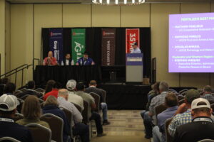
An educational panel on fertilizer best management practices in vine, tree nut and stone fruit crops caught the attention of attendees at this year’s Crop Consultant Conference.
Distinguished Service Award
Presented for the first time this year, the Distinguished Service Award honors the career of a retiring CCA in the western region. The inaugural winner was Fred Strauss, one of the first to get certified upon the 1992 founding of the CCA program.
Strauss was 1991 Member of the Year for the California Association of Pest Control Advisers; a WRCCA board member, including past board chair and marketing committee chair; and showed continued engagement in the industry after retirement, including volunteering with the International Certified Crop Adviser Board.
“Fred has been in ag for a very long time,” Vasquez said. “He’s mentored a lot of people. But the most important thing is that he’s been a friend to everyone, and he’s really done Western Region CCA a wonderful service and has really put it on a path for future success.”
“I want to thank the board,” Strauss said. “This is a great honor. And to be the first, that’s a big deal.”
On behalf of the JCS Marketing Inc. team and Progressive Crop Consultant magazine, the editor would like to thank all that attended this year’s Crop Consultant Conference in Visalia. The conference was a success with over 600 attendees who enjoyed the valuable seminars, exhibitors, networking and food.
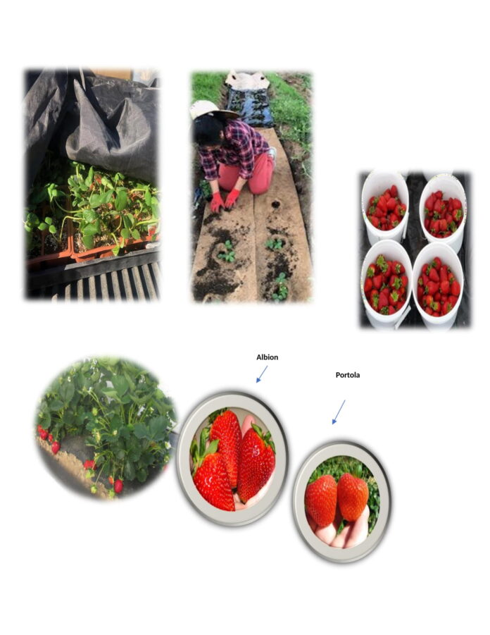
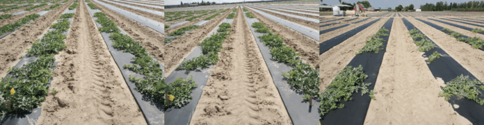
Trials set up for biodegradable mulch use at day 1 and harvesting.
Plastic film is widely used in crop production; however, growing environmental concerns call for reducing plastic waste. Biodegradable and bio-based mulches have emerged as promising alternatives that support sustainable agriculture. Small farms often prioritize sustainability and seek to reduce plastic waste in soil and food systems, particularly when bio-based mulches can match or exceed the benefits of traditional plastic mulch. However, limited data exist on the effectiveness of biodegradable paper and bio-based film in small-scale crop production, especially in areas frequently affected by heat and drought stress (Deschamps et al. 2021). Few studies have examined whether these bio-based films can competitively influence yield and fruit quality compared to standard plastic film.
Testing Five Mulch Treatments A field experiment was conducted in a strawberry field in Redlands, San Bernardino County, California with two goals in mind:
• Investigate the impact of different mulch types on soil temperature, fruit yield and fruit quality at harvest.
• Identify the most appropriate bio-based film regarding yield and quality for growing day-neutral strawberries in a Mediterranean climate for the Inland Empire region.
The project began in 2024 and is now in its second growing season. The trial followed a randomized complete split-plot design with five treatments commonly used by small farms in California: polyethylene mulch, landscape paper mulch, coconut liner mulch, biodegradable plastic mulch and bare soil (control). The everbearing strawberry variety Albion was planted with 20 plants per plot, and each treatment was replicated three times. Mature fruit (90% to 100% red) was harvested twice weekly to measure total and marketable yield (fruit without defects). Three harvests were evaluated for fruit quality.
To assess the suitability and performance of each mulch type, soil properties (temperature, moisture and pH) were recorded daily. Fruit yield (fruit weight and number of fruits per plant) was measured biweekly, and fruit quality (soluble solids (degrees Brix) and color parameters (L* = lightness; a* = redness)) was evaluated at harvest, reflecting farm stand and U-pick market standards.
Statistical Models for Yield and Quality Metrics Data were analyzed using SAS software, version 9.4 (SAS Institute Inc., Cary, N.C.). Normality was tested using PROC REG and PROC UNIVARIATE. Fruit yield data were analyzed using a linear mixed model (PROC GLIMMIX), and mean separation was conducted using the least significant difference (LSD) test. Fruit quality across three harvests was evaluated with PROC GLIMMIX, considering cultivar, mulch, year, time and their interactions as fixed effects, as well as harvest as a random effect. For day 0, fruit quality, cultivar, mulch film and their interaction were included as fixed effects in PROC GLIMMIX.
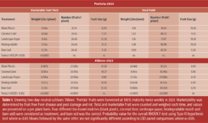
Coconut and Biodegradable Mulches Boost Yields In 2024, there were significant treatment effects on total and marketable fruit yield (Table 1). Strawberries grown with the coconut liner mulch produced significantly higher total fruit yield (pounds per plant) compared to the other plastic mulch treatments.
Total and marketable fruit weight per plant was 38% and 33% higher, respectively, for plants grown with coconut liner and biodegradable mulch compared to bare soil (P < 0.0001). The black plastic and landscape paper mulches resulted in similar total and marketable yields (fruit weight per plant) to those grown on bare soil.
Table 1. Showing two-day-neutral cultivars ‘Albion’, ‘Portola’ fruits were harvested at 100% maturity twice weekly in 2023. Marketability was determined by fruit free from disease and pest damage and rot. Total and marketable fruit were counted and weighed each time, and values are presented on a per plant basis. Four different bio-based mulches (black plastic, coconut liner, landscape paper, biodegradable mulch and bare soil) were considered as treatment, and bare soil was the control. Probability value for the overall ANOVA F-test using Type III hypothesis test where α=0.05 Means followed by the same letter are not significantly different according to LSD paired comparisons where α=0.05.
Fruit Size and Sweetness Show Minimal Mulch Influence No significant differences were observed in total or marketable fruit size among mulch treatments during either production year. Similarly, no significant treatment or interaction effects were found for fruit quality (soluble solids content, degrees Brix) compared with bare soil. Soluble solids content at harvest was significantly affected only by cultivar (P < 0.0001). Albion strawberries had 31% higher degrees Brix than Portola; however, there were no significant differences in degrees Brix among mulches within either cultivar (Table 2).
Table 2. A linear mixed model was used to test which factors and interactions had significant effects on the examined quality parameter (P ≤ 0.05). The effects of mulch on fruit quality measured only at day of harvest were not significant.
Coconut liner and biodegradable mulches resulted in the highest increase in marketable fruit weight compared to other treatments. Albion showed significantly higher soluble solids content (degrees Brix) when grown with coconut liner and biodegradable mulches; however, varietal effects on fruit composition were also evident across treatments.
Overall, the use of biodegradable mulch showed a trend toward higher yield and improved quality in day-neutral strawberry varieties grown under trenching or hillside production systems.
This research was funded by JEHOVAH JIREH F Mobile Farm and UCCE. The author would like to thank JJM farm for allocating the field to conduct this trial.
References
Deschamps, S. S., & Agehara, S. (2021). Metalized-striped plastic mulch reduces root-zone temperatures during establishment and increases early-season yields of annual winter strawberry. HortScience, 54(1), 110–116.
Salem, A. A., & Helaly, A. A. (2019). Impact of mycorrhizae and polyethylene mulching on growth, yield, and seed oil production of bottle gourd (Lagenaria siceraria). Journal of Horticultural Science & Ornamental Plants, 9, 28–38.
Sharma, S., Pant, P., Sangwan, M., & Sahrawat, R. (2024). Effect of organic and inorganic mulch on growth, yield, and quality of strawberry cv. Winter Dawn. International Journal of Environment and Climate Change, 14(3), 377–382.
Luminare, M.-C., Iaco Mi, B., Szilagyi, L., & Cristea, S. (2024). Research on the impact of the mulching system on strawberry yield. ResearchGate.
Ahmed, M., Duis, K. E., & Coors, A. (2024). Microplastics in the aquatic and terrestrial environment: Sources, fate, and effects. Environmental Sciences Europe, 28(1), 1–25.
Figure 1. Plant population comparisons for different in-row spacings. 3 feet apart = 2,100 plants/acre (left);
4.5 feet apart = 1,450 plants/acre (30% reduction) (middle); and 6 feet apart = 1,050 plants/acre (50% reduction) (right).
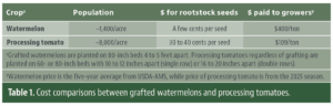
Research on grafted watermelonsin California has entered its seventh year since 2019. As adoption grows in acreage, economic gains and yield advantage, there is a need to review the development of watermelon grafting research, consider emerging issues and offer reliable production guidance to those new to this practice. The goal is to support long-term sustainability and viability of watermelon production in California.
Grafted watermelon acreage in California is about 2,500 acres in the 2024 season, 15 times more than in 2019. Many people are surprised and ask, “Why has acreage grown so fast? And why watermelon rather than tomato, given that tomatoes are more familiar in grafting contexts?” The answers are multifaceted.
First, watermelon fields use far fewer plants per acre than tomato (fresh market or processing), which lowers the cost of grafted transplants. Second, rootstock seed for watermelon is cheaper than that for tomato. Third, watermelon is a higher-value crop compared to tomatoes, especially processing tomatoes. Lower transplant cost, cheaper rootstock seed and higher grower returns combine to form a clear pathway to profitability for grafted watermelons. The table below compares cost categories for grafted watermelon vs processing tomato.
We divided the development of watermelon grafting research into four overlapping phases.
Table 1. Cost comparisons between grafted watermelons and processing tomatoes.
Phase 1: Identify Optimal Growing Practices for Grafted Watermelons, Spacing (2019-21) Because the high cost of grafted transplants is a key barrier to adoption in commercial systems, we prioritized reducing plant density while maintaining yield and quality. From 2019 to 2021, on-farm experiments evaluated multiple in-row spacings (3, 4, 5 and 6 feet) for full-size grafted watermelons (Fig. 1). An in-row spacing of 4.5 feet became the industry standard. At that spacing, each acre needs only 1,400 plants, 35% fewer than in nongrafted production, without a drop in yield. We also performed economic analyses illustrating when growers achieve profitability under each spacing (Wang and Fulford 2021).
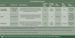
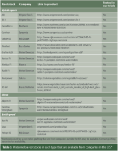
Phase 2: Understand Rootstock Characteristics and Field Performance (2021-25) After identifying optimal spacing, we responded to grower needs by screening rootstocks and scions suited to California’s conditions. Since 2021, on-farm trials have tested combinations of rootstocks and scions across commercial fields. More than 10 interspecific hybrid squash, citron and bottle gourd rootstocks were evaluated for yield, fruit quality and cost. Simultaneously, scion varieties differing in maturity, rind traits and shape were grafted onto locally popular rootstocks to test compatibility, yield, fruit quality and marketability. The two tables below summarize key characteristics of three rootstock types and their field performance, along with examples of rootstocks available from U.S. companies (Tables 2 and 3). For the full list of cucurbit rootstocks (including non-U.S.), see vegetablegrafting.org/resources/rootstock-tables/cucurbit-rootstocks/.
Table 2. Key characteristics of three types of rootstocks and their field performance from on-farm trials in California.Table 3. Watermelon rootstocks in each type that are available from companies in the U.S.*
Phase 3: Nitrogen and Irrigation Demand for Grafted Watermelons (2021-25) As rootstock and scion combinations began showing yield and quality advantages, growers explored how irrigation and nutrient, especially nitrogen, application should change for grafted watermelons given their differing growth patterns. The consecutive years of drought in California’s Central Valley have made irrigation management more challenging. Using smart irrigation tools allows growers to apply water based on actual crop needs. Since 2021, we have conducted on-farm experiments using the online decision-support tool CropManage to guide sustainable irrigation and N management for grafted watermelon with backing from the National Watermelon Association (Wang et al. 2024). We observed distinct N uptake patterns in grafted vs nongrafted plants, indicating the need to adjust applications to maintain productivity (Wang and Fulford 2022).
In the 2024 field trial, plant tissue nitrate declined sharply from June 20 to July 18 for both grafted and nongrafted plants. This was a sign of nitrate translocation from vegetative tissue to fruit. During that period, plants slowed nitrate uptake, resulting in either slight rises or steady soil nitrate levels. However, soil nitrate in nongrafted plots rose sharply, indicating accumulation from fertigation inputs. After July 18, continual N fertilization intended to promote vine regrowth and fruiting led to slight increases in tissue nitrate in grafted plants, with soil nitrate either rising or holding steady. Nongrafted vines, having entered senescence, showed decreasing tissue nitrate content.
For canopy coverage, which is key to estimating crop coefficient and evapotranspiration (ET), vines grew rapidly early. After the first harvest (July 10, 2024), canopy coverage fell, then recovered slowly and leveled off later. Grafted plant canopies (CAM and COB) followed that pattern. Nongrafted plot canopies declined most sharply and were the lowest through August 2024. Consequently, growers should understand how grafted watermelons use nutrients and water and tailor applications to their higher post-grafting vigor.
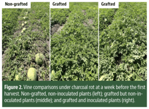
Figure 2. Vine comparisons under charcoal rot at a week before the first harvest. Non-grafted, non-inoculated plants (left); grafted but non-inoculated plants (middle); and grafted and inoculated plants (right).
Phase 4: Grafting as a Tool to Enable Other Sustainable Practices (2022-25) Although subsurface drip irrigation is widely used for watermelon in California and the region’s dry growing season suppresses some soilborne pathogens, such as fusarium and verticillium wilt, other diseases like charcoal rot (Macrophomina phaseolina) pose risk under hot dry conditions. Rising fumigation costs and restricted pesticide use have spurred interest in combining grafting with biological control. Since 2022, we have collaborated with the California Department of Pesticide Regulation to test combinations of grafting and Trichoderma biofungicides to reduce dependence on soil fumigants while maintaining yield and plant health. We compared application methods (tray drenching vs soil chemigation), Trichoderma formulations, rootstock choices and their interactions. We observed yield benefits from using Trichoderma and rootstocks both individually and synergistically (Buojaylah and Wang 2024; Buojaylah et al. 2024). Grafting and drenching with Trichoderma effectively managed charcoal rot (Fig. 5). These results support grafting as a reliable way to prevent vine decline and boost yield, and they inform best practices for biofungicide use. The research favors applying Trichoderma in the nursery to maximize microbial colonization and efficacy. Many vegetable growers are beginning to adopt that method as a routine practice.
Looking Ahead: Questions to Be Answered • How can we accurately estimate fruit maturity delay after grafting? As more rootstocks become commercialized, predicting maturity and any delay becomes more complex. A grafted fruit may remain immature even when classical indicators such as tendril, vine and rind suggest maturity.
• What is the pathogen load threshold beyond which rootstock effects are negated? That remains hard to determine since rootstock choice, grafted plant vigor and abiotic stress all influence disease resistance. We have seen grafted plants afflicted with symptoms of Fusarium wilt and other soilborne pathogens.
• How should we strategically select pollenizers? The interactions among pollenizers, rootstocks and scions and their effects on fruit maturity and quality remain less understood.
• Can grafting work equally well on other types of watermelon? We are beginning to explore whether grafting mini watermelons or specialty types such as yellow-flesh yields results comparable to full-size red-flesh varieties.
References Wang, Z., and Fulford, A. (2021). Is there a pathway to profitability for grafted watermelon? Vegetables West. 25, 8-10 https://vegetableswest.com/2021/09/01/read-september-october-2021-issue/.
Wang, Z., and Fulford, A. (2022). Nitrogen fertilization for grafted & non-grafted watermelons: Case study demonstrates different yield response. Vegetables West. 25, 10-12 https://vegetableswest.com/2022/09/01/read-sept-oct-2022-issue/.
Buojaylah, F., and Wang, Z. (2024). Two-year summary: Impacts of grafting and Trichoderma biofungicide on watermelon productivity and plant health. The Adviser-CAPCA. 27, 42-46 https://capca.com/wp-content/uploads/2024/03/CAPCA_ADV_APR-2024_LowRes.pdf.
Buojaylah, F., Castrejon, Y., and Wang, Z. (2024). Evaluating Trichoderma-containing biofungicide and grafting for productivity and plant health of triploid seedless watermelon in California’s commercial production. HortScience. 59, 1709-1717. https://doi.org/10.21273/HORTSCI18048-24.
Wang, Z., Cahn, M., and Buojaylah, F. (2024). Application of CropManage for processing tomato and watermelon production in the northern San Joaquin Valley. Progressive Crop Consultant. 9, 28-33 http://publications.myaglife.com/books/qjqd/#p=1.
LOVELAND, CO (November 12, 2025) –Loveland Products, Inc., announces that TITAN® XC, its leading fertilizer biocatalyst, has now been applied to more than 100 million acres across North America since its introduction in 2013. The achievement marks a significant milestone, underscoring TITAN XC’s long-standing role in helping farmers maximize nutrient efficiency, improve fertilizer performance, and achieve consistent, field-proven results year after year.
“Reaching 100 million acres isn’t just about scale – it’s about the success stories behind every acre,” says Ron Calhoun, Senior Plant Nutrition Portfolio Manager, with Loveland Products. “From early adopters to first-time users, farmers continue to tell us how TITAN XC helps them get more out of every ton of fertilizer, every acre, and every season.”
Proven Performer for Dry Fertilizer Programs TITAN XC is specifically formulated for dry fertilizer blends and leverages concentrated biochemistry to improve nutrient availability and uptake. By accelerating the mineralization of treated dry fertilizers and converting organic nutrients into plant-available inorganic states, TITAN XC enhances early root growth and maximizes the value of phosphorus and potassium applications.
TITAN XC Agronomic Benefits
Accelerates nutrient availability from applied dry fertilizers
Improves nutrient uptake by enhancing soil-fertilizer interaction for greater efficiency
Promotes stronger root development through improved nutrient uptake and utilization
Optimizes yield potential for a higher return on fertilizer investment
“TITAN XC changes the way that dry fertilizer responds to soil,” Calhoun explains. “The unique and concentrated biochemistry in TITAN XC provides the broadest range of activity across phosphorus, potassium, sulfur, and other nutrients to maximize the return on your fertilizer investment.”
TITAN XC integrates seamlessly into both fall and spring dry-fertilizer programs and works effectively across a wide range of soils and cropping systems without requiring special equipment or additional field passes. “With TITAN XC, farmers can stay in their normal fertility rhythm and still enhance fertilizer performance,” he notes.
Delivering Measurable Value TITAN XC has built a track record of reliability and consistent performance. “TITAN XC unlocks applied nutrients more quickly, supporting steady growth and dependable results,” says Calhoun. “That reliability is why farmers continue to choose it year after year.”
For those farmers still considering post-harvest fertilizer applications, Calhoun says TITAN XC offers a clear advantage.
“By improving nutrient availability and optimizing fertilizer efficiency, TITAN XC allows farmers to maximize the value of every pound of fertilizer applied, strengthen root systems ahead of winter, and set the stage for a productive spring,” he says. “It’s proven consistency and broad-spectrum activity make it an ideal choice for growers looking to protect their fertilizer investment and achieve more predictable outcomes across variable soils and conditions.”
With 100 million acres treated and counting, TITAN XC remains one of the most trusted and widely adopted fertilizer enhancement technologies in agriculture today. Loveland Products is proud to support Nutrien Ag Solutions farmer customers with innovations like TITAN XC that deliver consistent performance, measurable value, and long-term soil health benefits.
For more information on TITAN XC, reach out to your local Nutrien Ag Solutions crop consultant, or go to www.lovelandproducts.com/titanxc.
###
About Nutrien Ag Solutions and Loveland Products, Inc. Nutrien Ag Solutions®, Inc., the retail division of Nutrien Ltd., is a global leader in providing crop inputs and services. Through a network of over 4,500 trusted crop consultants, they offer full-acre solutions, helping farmers achieve the highest yields. Their product selection includes proprietary brands like Loveland Products®, Inc., Proven® Seed, and Dyna-Gro® Seed. Loveland Products offers a comprehensive line of high-performance input products. Their portfolio includes seed treatment, plant nutrition, fertilizer, adjuvant, and crop protection products, all highly respected in the industry. They constantly strive to introduce new, unique chemistries to the marketplace to provide innovative solutions to challenges across agricultural and professional non-crop industries. For more information, visit nutrienagsolutions.com and lovelandproducts.com.


 Invading California")

